6.824
W1 MapReduce, RPC & threads
Lecture 1
Labs
- Lab 1: MapReduce
- Lab 2: replication for fault-tolerance using Raft
- Lab 3: fault-tolerant key/value store
- Lab 4: sharded key/value store
Main Topics
This is a course about infrastructure for applications.
- Storage.
- Communication.
- Computation.
Topic: implementation
- RPC, threads, concurrency control.
Topic: performance
- The goal: scalable throughput
- Nx servers -> Nx total throughput via parallel CPU, disk, net.
- [diagram: users, application servers, storage servers]
- So handling more load only requires buying more computers rather than re-design by expensive programmers.
- Effective when you can divide work w/o much interaction.
Topic: fault tolerance
We often want:
- Availability – app can make progress despite failures
- Recoverability – app will come back to life when failures are repaired
Big idea: replicated servers.
- If one server crashes, can proceed using the other(s).
- Labs 1, 2 and 3
Topic: consistency
General-purpose infrastructure needs well-defined behavior.
E.g. “
Get(k)yields the value from the most recentPut(k,v).”
$$
\begin{cases}
Put(k,v) \
Get(k)
\end{cases}
$$
Achieving good behavior is hard!
- “Replica” servers are hard to keep identical.
- Clients may crash midway through multi-step update.
- Servers may crash, e.g. after executing but before replying.
- Network partition may make live servers look dead; risk of “split brain”.
Consistency and performance are enemies.
Strong consistency requires communication,
e.g.
Get()must check for a recentPut().Many designs provide only weak consistency, to gain speed.
e.g. Get() does not yield the latest Put()!
Painful for application programmers but may be a good trade-off.
Many design points are possible in the consistency/performance spectrum!
CASE STUDY: MapReduce
MapReduce overview
context: multi-hour computations on multi-terabyte data-sets
e.g. build search index, or sort, or analyze structure of web
- only practical with 1000s of computers
- applications not written by distributed systems experts
overall goal: easy for non-specialist programmers
programmer just defines Map and Reduce functions: often fairly simple sequential code
MR takes care of, and hides, all aspects of distribution!
Abstract view of a MapReduce job
input is (already) split into M files
1 | Input1 -> Map -> a,1 b,1 |
MR calls Map() for each input file, produces set of $<k2,v2>$
- “intermediate” data
- each
Map()call is a “task”
MR gathers all intermediate $v2$’s for a given $k2$, and passes each key + values to a Reduce call
final output is set of $<k2,v3>$ pairs from Reduce()s
Example: word count : input is thousands of text files
1 | Map(k, v) |
MapReduce scales well:
$N$ “worker” computers get you $Nx$ throughput.
- Maps()s can run in parallel, since they don’t interact.
- Same for Reduce()s.
So you can get more throughput by buying more computers.
MapReduce hides many details:
- sending app code to servers
- tracking which tasks are done
- moving data from Maps to Reduces
- balancing load over servers
- recovering from failures
However, MapReduce limits what apps can do:
- No interaction or state (other than via intermediate output).
- No iteration, no multi-stage pipelines.
- No real-time or streaming processing.
Input and output are stored on the GFS cluster file system
MR needs huge parallel input and output throughput.
GFS splits files over many servers, in 64 MB chunks
- Maps read in parallel
- Reduces write in parallel
GFS also replicates each file on 2 or 3 servers
Having GFS is a big win for MapReduce
What will likely limit the performance?
We care since that’s the thing to optimize. CPU? memory? disk? network?
In 2004 authors were limited by network capacity —— What does MR send over the network?
- Maps read input from GFS.
- Reduces read Map output :Can be as large as input, e.g. for sorting.
- Reduces write output files to GFS.
[diagram: servers, tree of network switches]
In MR’s all-to-all shuffle, half of traffic goes through root switch.
Paper’s root switch: 100 to 200 gigabits/second, total
- 1800 machines, so 55 megabits/second/machine.
- 55 is small, e.g. much less than disk or RAM speed.
Today: networks and root switches are much faster relative to CPU/disk.
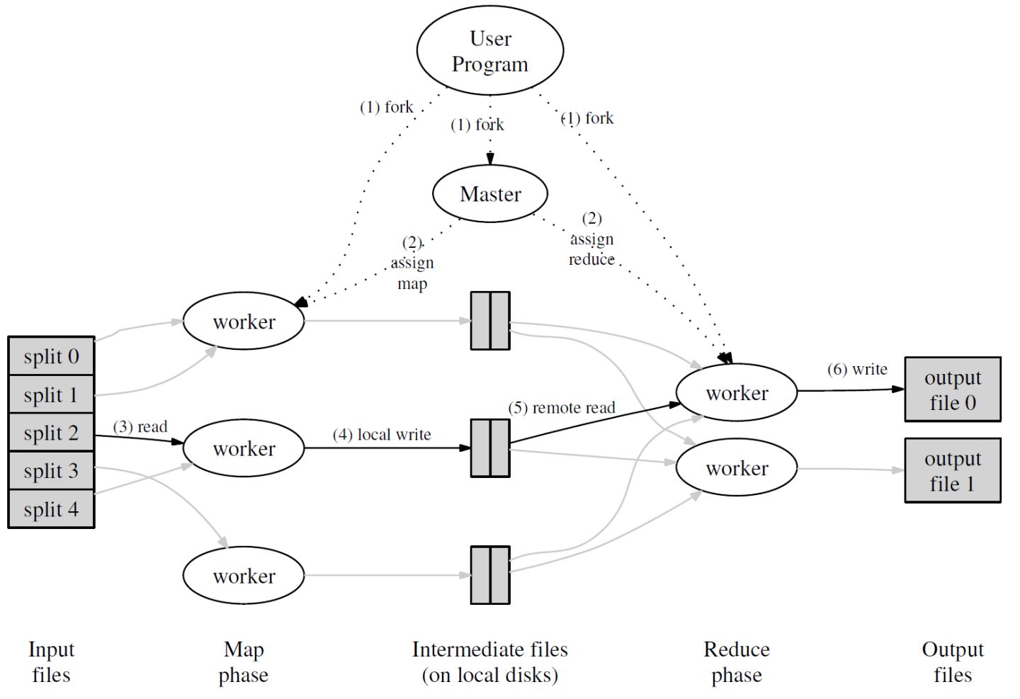
Some details (paper’s Figure 1):
one master, that hands out tasks to workers and remembers progress.
master gives Map tasks to workers until all Maps complete
Maps write output (intermediate data) to local disk
Maps split output, by hash, into one file per Reduce task
after all Maps have finished, master hands out Reduce tasks
each Reduce fetches its intermediate output from (all) Map workers
each Reduce task writes a separate output file on GFS
How does MR minimize network use?
Master tries to run each Map task on GFS server that stores its input.
- All computers run both GFS and MR workers
- So input is read from local disk (via GFS), not over network.
Intermediate data goes over network just once.
- Map worker writes to local disk.
- Reduce workers read directly from Map workers, not via GFS.
Intermediate data partitioned into files holding many keys.
- R is much smaller than the number of keys.
- Big network transfers are more efficient.
How does MR get good load balance?
Wasteful and slow if N-1 servers have to wait for 1 slow server to finish.
But some tasks likely take longer than others.
Solution: many more tasks than workers.
- Master hands out new tasks to workers who finish previous tasks.
- So no task is so big it dominates completion time (hopefully).
- So faster servers do more tasks than slower ones, finish abt the same time.
What about fault tolerance?
I.e. what if a worker crashes during a MR job?
We want to completely hide failures from the application programmer!
Does MR have to re-run the whole job from the beginning? Why not?
- MR re-runs just the failed Map()s and Reduce()s.
- Suppose MR runs a Map twice, one Reduce sees first run’s output, —— another Reduce sees the second run’s output?
- Correctness requires re-execution to yield exactly the same output.
- So Map and Reduce must be pure deterministic functions:
- they are only allowed to look at their arguments.
- no state, no file I/O, no interaction, no external communication.
What if you wanted to allow non-functional Map or Reduce?
- Worker failure would require whole job to be re-executed, or you’d need to create synchronized global checkpoints.
Details of worker crash recovery:
- Map worker crashes:
- master notices worker no longer responds to pings
- master knows which Map tasks it ran on that worker
- those tasks’ intermediate output is now lost, must be re-created
- master tells other workers to run those tasks
- can omit re-running if Reduces already fetched the intermediate data
- Reduce worker crashes.
- finished tasks are OK – stored in GFS, with replicas.
- master re-starts worker’s unfinished tasks on other workers.
Other failures/problems:
- What if the master gives two workers the same Map() task?
- perhaps the master incorrectly thinks one worker died.
- it will tell Reduce workers about only one of them.
- What if the master gives two workers the same Reduce() task?
- they will both try to write the same output file on GFS!
- atomic GFS rename prevents mixing; one complete file will be visible.
- What if a single worker is very slow – a “straggler”?
- perhaps due to flakey hardware.
- master starts a second copy of last few tasks.
- What if a worker computes incorrect output, due to broken h/w or s/w?
- too bad! MR assumes “fail-stop” CPUs and software.
- What if the master crashes?
Current status?
- Hugely influential (Hadoop, Spark, &c).
- Probably no longer in use at Google.
- Replaced by Flume / FlumeJava (see paper by Chambers et al).
- GFS replaced by Colossus (no good description), and BigTable.
Conclusion
MapReduce single-handedly made big cluster computation popular.
“-” Not the most efficient or flexible.
“+” Scales well.
“+” Easy to program – failures and data movement are hidden.
These were good trade-offs in practice.
Lecture 2: Infrastructure: RPC and threads
Why Go?
- good support for threads
- convenient RPC
- type- and memory- safe
- garbage-collected (no use after freeing problems)
- threads + GC is particularly attractive!
- not too complex
After the tutorial, use https://golang.org/doc/effective_go.html
Threads
- a useful structuring tool, but can be tricky
- Go calls them goroutines; everyone else calls them threads
Thread = “thread of execution”
- threads allow one program to do many things at once
- each thread executes serially, just like an ordinary non-threaded program
- the threads share memory
- each thread includes some per-thread state:
- program counter,
- registers,
- stack,
- what it’s waiting for
Why threads?
I/O concurrency
- Client sends requests to many servers in parallel and waits for replies.
- Server processes multiple client requests; each request may block.
- While waiting for the disk to read data for client X,
- process a request from client Y.
Multicore performance
- Execute code in parallel on several cores.
Convenience
- In background, once per second, check whether each worker is still alive.
Is there an alternative to threads?
“event-driven.”
write code that explicitly interleaves activities, in a single thread. Usually called “event-driven.”
Keep a table of state about each activity, e.g. each client request.
One “event” loop that:
- checks for new input for each activity (e.g. arrival of reply from server),
- does the next step for each activity,
- updates state.
Event-driven gets you I/O concurrency, and eliminates thread costs (which can be substantial), but doesn’t get multi-core speedup, and is painful to program.
Threading challenges:
sharing data safely
what if two threads do n = n + 1 at the same time?
- or one thread reads while another increments?
this is a “race” – and is often a bug
-> use locks (Go’s sync.Mutex)
-> or avoid sharing mutable data
coordination between threads
one thread is producing data, another thread is consuming it
- how can the consumer wait (and release the CPU)?
- how can the producer wake up the consumer?
-> use Go channels or sync.Cond or sync.WaitGroup
deadlock
cycles via locks and/or communication (e.g. RPC or Go channels)
Let’s look at the tutorial’s web crawler as a threading example.
What is a web crawler?
- goal: fetch all web pages, e.g. to feed to an indexer
- you give it a starting web page
- it recursively follows all links
- but don’t fetch a given page more than once
- and don’t get stuck in cycles
Crawler challenges
Exploit I/O concurrency
- Network latency is more limiting than network capacity
- Fetch many URLs at the same time
- To increase URLs fetched per second
- => Use threads for concurrency
Fetch each URL only once
- avoid wasting network bandwidth
- be nice to remote servers
- => Need to remember which URLs visited
Know when finished
We’ll look at three styles of solution [crawler.go on schedule page]
Serial crawler
- performs depth-first exploration via recursive Serial calls
- the “fetched” map avoids repeats, breaks cycles
- a single map, passed by reference, caller sees callee’s updates
- but: fetches only one page at a time – slow
- can we just put a “go” in front of the Serial() call?
- let’s try it… what happened?
Concurrent Mutex crawler
- Creates a thread for each page fetch
- Many concurrent fetches, higher fetch rate
- the “go func” creates a goroutine and starts it running
- func… is an “anonymous function”
- The threads share the “fetched” map
- So only one thread will fetch any given page
- Why the Mutex (Lock() and Unlock())?
- One reason:
- Two threads make simultaneous calls to ConcurrentMutex() with same URL
- Due to two different pages containing link to same URL
- T1 reads fetched[url], T2 reads fetched[url]
- Both see that url hasn’t been fetched (already == false)
- Both fetch, which is wrong
- The mutex causes one to wait while the other does both check and set
- So only one thread sees already==false
- We say “the lock protects the data”
- But not Go does not enforce any relationship between locks and data!
- The code between lock/unlock is often called a “critical section”
- Two threads make simultaneous calls to ConcurrentMutex() with same URL
- Another reason:
- Internally, map is a complex data structure (tree? expandable hash?)
- Concurrent update/update may wreck internal invariants
- Concurrent update/read may crash the read
- What if I comment out Lock() / Unlock()?
- go run crawler.go
- Why does it work?
- go run -race crawler.go
- Detects races even when output is correct!
- go run crawler.go
- One reason:
- How does the ConcurrentMutex crawler decide it is done?
- sync.WaitGroup
- Wait() waits for all Add()s to be balanced by Done()s
- i.e. waits for all child threads to finish
- [diagram: tree of goroutines, overlaid on cyclic URL graph]
- there’s a WaitGroup per node in the tree
- How many concurrent threads might this crawler create?
ConcurrentMutex crawler
a Go channel:
a channel is an object
1
ch := make(chan int)
a channel lets one thread send an object to another thread
1
ch <- x
the sender waits until some goroutine receives, a receiver waits until some goroutine sends
1 | y := <- ch |
- channels both communicate and synchronize
- several threads can send and receive on a channel
- channels are cheap
- remember: sender blocks until the receiver receives!
- “synchronous”
- watch out for deadlock
ConcurrentChannel coordinator()
- coordinator() creates a worker goroutine to fetch each page
- woker() sends slice of page’s URLs on a channel
- multiple workers send on the single channel
- coordinator() reads URL slices from the channel
At what line does the coordinator wait?
- Does the coordinator use CPU time while it waits?
Note: there is no recursion here; instead there’s a work list.
Note: no need to lock the fetched map, because it isn’t shared!
How does the coordinator know it is done?
- Keeps count of workers in n.
- Each worker sends exactly one item on channel.
Why is it safe for multiple threads use the same channel?
Worker thread writes url slice, coordinator reads it, is that a race?
- worker only writes slice before sending
- coordinator only reads slice after receiving
So they can’t use the slice at the same time.
Why does ConcurrentChannel() create a goroutine just for “ch <- …”?
- Let’s get rid of the goroutine…
When to use sharing and locks, versus channels?
- Most problems can be solved in either style
- What makes the most sense depends on how the programmer thinks
- state – sharing and locks
- communication – channels
- For the 6.824 labs, I recommend sharing+locks for state,
- and
sync.Condor channels ortime.Sleep()for waiting/notification.
- and
Remote Procedure Call (RPC)
- a key piece of distributed system machinery; all the labs use RPC
- goal: easy-to-program client/server communication
- hide details of network protocols
- convert data (strings, arrays, maps, &c) to “wire format”
- portability / interoperability
RPC message diagram:
| Client | Server | |
|---|---|---|
| request | —> | |
| <— | response |
Software structure
| client app | handler fns | |
|---|---|---|
| stub fns | —> | dispatcher |
| RPC lib | RPC lib | |
| net | —— | net |
Go example: kv.go on schedule page
- A toy key/value storage server – Put(key,value), Get(key)->value
- Uses Go’s RPC library
- Common:
- Declare Args and Reply struct for each server handler.
- Client:
- connect()’s Dial() creates a TCP connection to the server
- get() and put() are client “stubs”
- Call() asks the RPC library to perform the call
- you specify server function name, arguments, place to put reply
- library marshalls args, sends request, waits, unmarshalls reply
- return value from Call() indicates whether it got a reply
- usually you’ll also have a reply.Err indicating service-level failure
- Server:
- Go requires server to declare an object with methods as RPC handlers
- Server then registers that object with the RPC library
- Server accepts TCP connections, gives them to RPC library
- The RPC library
- reads each request
- creates a new goroutine for this request
- unmarshalls request
- looks up the named object (in table create by Register())
- calls the object’s named method (dispatch)
- marshalls reply
- writes reply on TCP connection
- The server’s Get() and Put() handlers
- Must lock, since RPC library creates a new goroutine for each request
- read args; modify reply
A few details:
- Binding: how does client know what server computer to talk to?
- For Go’s RPC, server name/port is an argument to Dial
- Big systems have some kind of name or configuration server
- Marshalling: format data into packets
- Go’s RPC library can pass strings, arrays, objects, maps, &c
- Go passes pointers by copying the pointed-to data
- Cannot pass channels or functions
RPC problem: what to do about failures?
e.g. lost packet, broken network, slow server, crashed server
What does a failure look like to the client RPC library?
- Client never sees a response from the server
- Client does not know if the server saw the request!
- [diagram of losses at various points]
- Maybe server never saw the request
- Maybe server executed, crashed just before sending reply
- Maybe server executed, but network died just before delivering reply
Simplest failure-handling scheme: “best-effort RPC”
Call()waits for response for a while- If none arrives, re-send the request
- Do this a few times
- Then give up and return an error
Q: is “best effort” easy for applications to cope with?
A particularly bad situation:
- client executes
Put("k", 10);Put("k", 20);
- both succeed
- what will Get(“k”) yield?
- [diagram, timeout, re-send, original arrives late]
Q: is best effort ever OK?
- read-only operations
- operations that do nothing if repeated
- e.g. DB checks if record has already been inserted
Better RPC behavior: “at-most-once RPC”
idea: client re-sends if no answer;
- server RPC code detects duplicate requests,
- returns previous reply instead of re-running handler
Q: how to detect a duplicate request?
client includes unique ID (XID) with each request
- uses same XID for re-send
server:
1
2
3
4
5
6if seen[xid]:
r = old[xid]
else
r = handler()
old[xid] = r
seen[xid] = true
some at-most-once complexities
- this will come up in lab 3
- what if two clients use the same XID?
- big random number?
- how to avoid a huge seen[xid] table?
- idea:
- each client has a unique ID (perhaps a big random number)
- per-client RPC sequence numbers
- client includes “seen all replies <= X” with every RPC
- much like TCP sequence #s and acks
- then server can keep O(# clients) state, rather than O(# XIDs)
- idea:
- server must eventually discard info about old RPCs or old clients
- when is discard safe?
- how to handle dup req while original is still executing?
- server doesn’t know reply yet
- idea: “pending” flag per executing RPC; wait or ignore
What if an at-most-once server crashes and re-starts?
- if at-most-once duplicate info in memory, server will forget
- and accept duplicate requests after re-start
- maybe it should write the duplicate info to disk
- maybe replica server should also replicate duplicate info
Go RPC is a simple form of “at-most-once”
- open TCP connection
- write request to TCP connection
- Go RPC never re-sends a request
- So server won’t see duplicate requests
- Go RPC code returns an error if it doesn’t get a reply
- perhaps after a timeout (from TCP)
- perhaps server didn’t see request
- perhaps server processed request but server/net failed before reply came back
What about “exactly once”?
unbounded retries plus duplicate detection plus fault-tolerant service
Lab 3
MapReduce Paper Read
0 Abstract
Users specify
- a map function that processes a key/value pair to generate a set of intermediate key/value pairs,
- a reduce function that merges all intermediate values associated with the same intermediate key.
Programs written in this functional style are automatically parallelized and executed on a large cluster of commodity machines.
Run-time system takes care of the details of
- partitioning the input data,
- scheduling the program’s execution across a set of machines,
- handling machine failures,
- managing the required intermachine communication.
1 Introduction
| Section | Content |
|---|---|
| 2 | basic programming model and gives several examples. |
| 3 | an implementation of the MapReduce interface tailored towards our cluster-based computing environment. |
| 4 | several refinements of the programming model that we have found useful. |
| 5 | has performance measurements of our implementation for a variety of tasks. |
| 6 | explores the use of MapReduce within Google including our experiences in using it as the basis for a rewrite of our production indexing system. |
| 7 | discusses related and future work. |
2 Programming Model
2.1 Counting Word
1 | map(String key, String value): |
- The
mapfunction emits each word plus an associated count of occurrences (just ‘1’ in this simple example).- The
reducefunction sums together all counts emitted for a particular word.
2.2 Types
$map(k1,v1)→list(k2,v2)$
$map(k2,list(v2))→list(v2)$
2.3 More Examples
- Distributed Grep: The map function emits a line if it matches a supplied pattern. The reduce function is an identity function that just copies the supplied intermedi- ate data to the output.
- Count of URL Access Frequency: The map function processes logs of web page requests and outputs $⟨URL, 1⟩$. The reduce function adds together all values for the same URL and emits a $⟨URL, total count⟩$ pair.
- Reverse Web-Link Graph: The map function outputs $⟨target,source⟩$ pairs for each link to a target URL found in a page named source. The reduce function concatenates the list of all source URLs as- sociated with a given target URL and emits the pair: $⟨target, list(source)⟩$
- Term-Vector per Host: A term vector summarizes the most important words that occur in a document or a set of documents as a list of $⟨word,frequency⟩$ pairs. The map function emits a $⟨hostname, term vector⟩$ pair for each input document (where the hostname is extracted from the URL of the document). The reduce function is passed all per-document term vectors for a given host. It adds these term vectors together, throwing away infrequent terms, and then emits a final $⟨hostname, term vector⟩$ pair.
- Inverted Index: The map function parses each docu- ment, and emits a sequence of $⟨word, document ID⟩$ pairs. The reduce function accepts all pairs for a given word, sorts the corresponding document IDs and emits a $⟨word,list(document ID)⟩$ pair.Thesetofalloutput pairs forms a simple inverted index. It is easy to augment this computation to keep track of word positions.
- Distributed Sort: The map function extracts the key from each record, and emits a $⟨key, record⟩$ pair. The reduce function emits all pairs unchanged. This computation depends on the partitioning facilities described in Section 4.1 and the ordering properties described in Section 4.2.
3 Implementation
3.1 Execution Overview
首先,用户通过 MapReduce 客户端指定 Map 函数和 Reduce 函数,以及此次 MapReduce 计算的配置,包括中间结果键值对的 Partition 数量 $R$ 以及用于切分中间结果的哈希函数 $hash$ 。
用户开始 MapReduce 计算后,整个 MapReduce 计算的流程可总结如下:
- 作为输入的文件会被分为 $M$ 个 Split,每个 Split 的大小通常在 16~64 MB 之间
- 如此,整个 MapReduce 计算包含 $M$ 个Map 任务和 $R$ 个 Reduce 任务。Master 结点会从空闲的 Worker 结点中进行选取并为其分配 Map 任务和 Reduce 任务
- 收到 Map 任务的 Worker 们(又称 Mapper)开始读入自己对应的 Split,将读入的内容解析为输入键值对并调用由用户定义的 Map 函数。由 Map 函数产生的中间结果键值对会被暂时存放在缓冲内存区中
- 在 Map 阶段进行的同时,Mapper 们周期性地将放置在缓冲区中的中间结果存入到自己的本地磁盘中,同时根据用户指定的 Partition 函数(默认为 $hash(key){,}mod{,}R$)。 将产生的中间结果分为 $R$ 个部分。任务完成时,Mapper 便会将中间结果在其本地磁盘上的存放位置报告给 Master
- Mapper 上报的中间结果存放位置会被 Master 转发给 Reducer。当 Reducer 接收到这些信息后便会通过 RPC 读取存储在 Mapper 本地磁盘上属于对应 Partition 的中间结果。在读取完毕后,Reducer 会对读取到的数据进行排序以令拥有相同键的键值对能够连续分布
- 之后,Reducer 会为每个键收集与其关联的值的集合,并以之调用用户定义的 Reduce 函数。Reduce 函数的结果会被放入到对应的 Reduce Partition 结果文件
实际上,在一个 MapReduce 集群中,Master 会记录每一个 Map 和 Reduce 任务的当前完成状态,以及所分配的 Worker。除此之外,Master 还负责将 Mapper 产生的中间结果文件的位置和大小转发给 Reducer。
值得注意的是,每次 MapReduce 任务执行时, $M$ 和 $R$ 的值都应比集群中的 Worker 数量要高得多,以达成集群内负载均衡的效果。
3.2 Master Data Structure
MASTER keeps several data structures. For each map task and reduce task, it stores
- the state (idle, in-progress, or completed),
- the identity of the worker machine (for non-idle tasks).
The master is the conduit through which the location of intermediate file regions is propagated from map tasks to reduce tasks. Therefore, for each completed map task, the master stores the locations and sizes of the $R$ intermediate file regions produced by the map task. Updates to this location and size information are received as map tasks are completed. The information is pushed incrementally to workers that have in-progress reduce tasks.
3.3 Fault Tolerance
由于 Google MapReduce 很大程度上利用了由 Google File System 提供的分布式原子文件读写操作,所以 MapReduce 集群的容错机制实现相比之下便简洁很多,也主要集中在任务意外中断的恢复上。
woker failure
master pings every worker periodically. If no response from a worker timely,
- the master marks the worker as failed.
- Any map tasks completed by the worker are reset back to their initial idle state, therefore eligible for scheduling on other workers.
- Any map/reduce task in progress on a failed worker is also reset to idle and eligible for rescheduling.
- Completed map tasks are re-executed on a failure because their output is stored on the local disk(s) of the failed machine and is therefore inaccessible.
- Completed reduce tasks do not need to be re-executed since their output is stored in a global file system.
- When a map task is executed first by $worker A$ and then later executed by $worker B$ (because $A$ failed), all workers executing reduce tasks are notified of the re-execution. Any reduce task that has not already read the data from $worker A$ will read the data from $worker B$.
MapReduce is resilient to large-scale worker failures.
- For example, during one MapReduce operation, network maintenance on a running cluster was causing groups of 80 machines at a time to become unreachable for several minutes.
The MapReduce master simply re-executed the work done by the unreachable worker machines, and continued to make forward progress, eventually completing the MapReduce operation.
任何分配给该 Worker 的 Map 任务,无论是正在运行还是已经完成,都需要由 Master 重新分配给其他 Worker,因为该 Worker 不可用也意味着存储在该 Worker 本地磁盘上的中间结果也不可用了。Master 也会将这次重试通知给所有 Reducer,没能从原本的 Mapper 上完整获取中间结果的 Reducer 便会开始从新的 Mapper 上获取数据。
如果有 Reduce 任务分配给该 Worker,Master 则会选取其中尚未完成的 Reduce 任务分配给其他 Worker。鉴于 Google MapReduce 的结果是存储在 Google File System 上的,已完成的 Reduce 任务的结果的可用性由 Google File System 提供,因此 MapReduce Master 只需要处理未完成的 Reduce 任务即可。
master failure
Master 结点在运行时会周期性地将集群的当前状态作为保存点(Checkpoint)写入到磁盘中。Master 进程终止后,重新启动的 Master 进程即可利用存储在磁盘中的数据恢复到上一次保存点的状态。
但是,整个 MapReduce 集群中只会有一个 Master 结点,因此 Master 失效的情况并不多见。
因此,如果主节点失败,我们当前的实现将中止MapReduce计算。
客户端可以检查此条件,并根据需要重试MapReduce操作。
semantics in the presence of failure
当 User-supplied $map$ 和 $reduce$ 运算符是其输入值的确定性函数时,我们的分布式实现将生成与整个程序的非错误顺序执行所产生的输出相同的输出。
- 我们依靠 $map$ 的原子提交和 $reduce$ 任务输出来实现此属性。每个正在进行的任务都会将其输出写入私有临时文件。
- $reduce$ 任务生成一个这样的文件,$map$ 任务生成 $R$ 这样的文件 (one per reduce task)。
- $map$ task 完成后,$worker$ 会向 $master$ 发送一条消息,并在消息中包含 R 临时文件的名称。
- 如果 $master$ 收到已完成的 $map$ task 的已完成消息,它将忽略该消息。否则,它将在 $master$ 的数据结构中记录 $R$ 文件的名称。
- 当 $reduce$ 的任务完成时,$reduce$ worker 会 atomically 将其临时输出文件重命名为最终输出文件。
- 如果在多台计算机上执行相同的 reduce 任务,则会对同一最终输出文件执行多个重命名调用。
- 我们依靠底层文件系统提供的原子重命名操作来保证最终的文件系统状态只包含一次执行 $reduce$ 任务时生成的数据。
我们的绝大多数 $map$ 和 $reduce$ operators 都是 Deterministic 的,在这种情况下
- 我们的 semantics 等同于顺序执行的事实使得程序员很容易推断出他们的程序的 behavior。当 $map$ 和/或 $reduce$ operators 是非确定性的时,我们提供较弱但仍然合理的语义。
- 在存在 non-deterministic operators 的情况下,特定的 reduce 任务 R1 的输出等效于由 non-deterministic program 的 sequential execution 生成的 R1 的输出。
然而,不同 reduce 任务 R2 的输出可以对应于由 non-deterministic program 的 different sequential execution 产生的 R2 的输出。考虑 Map 任务 $M$ 和 Reduce 任务 $R_1$ 和 $R_2$:
Let $e(Ri)$ be the execution of $R_i$ that committed (there is exactly one such execution).
The weaker semantics arise because $e(R_1)$ may have read the output produced by one execution of $M$ , and $e(R_2)$ may have read the output produced by a different execution of $M$ .出现较弱的语义是因为 $e(R1)$ 可能已读取由 $M$ 的一个执行产生的输出,而 $e(R2)$ 可能已读取由 $M$ 的不同执行产生的输出。
3.4 Locality
网络带宽资源相对稀缺,通过利用输入数据(GFS 管理)存储在组成集群的机器的本地磁盘上这一事实来节省网络带宽。GFS 将每个文件划分为 64MB 的块,并在不同的机器上存储每个块的多个副本(typically 3 个副本)。
MapReduce master 会考虑输入文件的位置信息,并尝试在包含相应输入数据副本的计算机上调度 map 任务。如果做不到这一点,它会尝试在该任务的输入数据的副本附近调度 map 任务
(e.g., on a worker machine that is on the same network switch as the machine containing the data)。
当对集群中很大一部分 wokers 运行大型 MapReduce 操作时,大多数输入数据都是在本地读取的,并且不消耗网络带宽。
3.5 Task Granularity
如上所述,我们将 map phase 细分为 $M$ 个部分,将 reduce phase 细分为 $R$ 个部分。
理想情况下,$M$ 和 $R$ 应比 worker machine 的数量大得多。让每个 woker 执行许多不同的任务可以改善动态负载平衡 (dynamic load balancing),还可以在一个 worker fails 时加快恢复速度:它已完成的许多 map 任务可以被分布在所有其他 worker machine 上。
在我们的实现中,$M$ 和 $R$ 的大小是有实际限制的,因为 master 必须做出 $O(M+R)$ 调度决策,并将 $O(MR)$ 状态保存在如上所述的内存中。(然而,constant factors for memory usage 很小:the $O(MR)$ piece of the state consists of approximately one byte of data per map task/reduce task pair)
此外,$R$ 通常受到用户的约束,因为每个 reduce 任务的输出最终都位于单独的 output 文件中。在实践中,我们倾向于选择 $M$,以便每个单独的任务大约是 16 MB 到 64 MB 的输入数据(以便上面描述的 locality optimization 局部性优化是最有效的),并且我们使 $R$ 成为我们期望使用的 worker machine 数量的 small multiple。We often perform MapReduce computations with $M=200,000$ and $R=5,000$, using $2,000$ worker machines.
3.6 Backup Tasks
“straggler”:
- 一个需要非常长的时间才能完成计算中最后几个 map 或 reduce 任务之一的 machine。
- 延长 MapReduce 操作所花费的总时间的常见原因之一
- 出现原因:
- 例如,磁盘损坏的计算机可能会遇到频繁的 correctable errors,将其读取性能从 $30MB/s$ 降低到 $1MB/s$。
- 集群调度系统可能已经在机器上调度了其他任务,导致它由于 CPU,内存,本地磁盘或网络工作带宽的竞争而执行 MapReduce 代码的速度更慢。
- machine initialization code 中的一个错误,导致 processor caches 被禁用:受影响的 machines上的计算速度减慢了一百倍以上。
Alleviation 通用机制:
当 MapReduce 操作接近完成时,master 会计划其余 in-progress task 的备份执行。每当 primary 或 backup executions 完成时,任务都会标记为已完成。
我们调整了此机制,使其通常将操作使用的计算资源增加不超过百分之几。我们发现这大大减少了完成大型MapReduce 操作的时间。
作为一个例子,the sort program described in Section 5.3 takes 44% longer to complete when the backup task mechanism is disabled.
4 Refinement
尽管简单编写 Map 和 Reduce 函数基本满足大多需求,但一些扩展很有用。
4.1 Partitoning Function
MapReduce 的用户指定他们想要的减少任务/输出文件的数量 $(R)$。Data gets partitioned across these tasks using a partitioning function on the intermediate key. A default partitioning function is provided that uses hashing (e.g. “$hash(key) \mod R$”)。这往往会导致相当均衡的 partitions。但是,在某些情况下,some other function of the key 对数据进行分区是很有用的。例如,有时 the output keys 是 URLs,and 我们希望 a single host 的 all entries 最终都位于同一 output file 中。
为了支持这种情况,MapReduce 库的用户可以提供 special partitioning function。例如,使用 “$hash(Hostname(urlkey))\mod R$” 作为 partitioning 函数会导致来自同一主机的所有 URLs 最终都位于同一输出文件中。
4.2 Ordering Guarantees
我们保证在给定分区中,中间键/值对按递增键顺序处理。这种排序保证使得每个分区生成一个排序的输出文件变得容易,当输出文件格式需要支持按键进行高效的随机访问查找时,或者输出的用户发现对数据进行排序很方便时,很有用。
4.3 Combiner Function
在某些情况下,每个 map 任务生成的 intermediate keys 都存在显著的重复,并且用户指定的 Reduce 函数是可交换和关联的。一个例子是字数统计示例。由于词频倾向于遵循 Zipf 分布,因此每个映射任务将生成数百或数千条 $<the,1>$ 形式的记录。所有这些计数将通过网络发送到单个 reduce 任务,然后通过 Reduce 函数相加以生成一个数字。我们允许用户指定一个可选的 Combiner 函数,该函数在通过网络发送数据之前对数据进行部分合并。
Combiner 函数在每台执行 map 任务的计算机上执行。通常使用相同的代码来实现 Combiner 和 reduce 函数。reduce 函数和Combiner 函数之间的唯一区别是 MapReduce 库如何处理函数的输出。reduce 函数的输出将写入最终的输出文件。Combiner 函数的输出将写入将发送到 reduce 任务的中间文件。
Partial combining 显著加快了某些类别的 MapReduce 操作。附录 A 包含一个使用 combiner 的示例。
4.4 Input and Output Types
MapReduce 库支持以几种不同的格式读取输入数据。
- 例如,“text” 模式输入将每行视为键/值对:键是文件中的偏移量,值是行的内容。
- 另一种常见的格式是存储按键排序的键/值对序列。每个输入类型实现都知道如何将自身拆分为有意义的范围,以便作为单独的
map任务进行处理(例如, text 模式的 range splitting 可确保 range splits 仅在行边界处发生)。
用户可以通过提供简单的 $x$ 接口的实现来添加对新输入类型的支持,尽管大多数用户只使用少量预定义输入类型中的一个。
A reader 不一定需要提供从文件读取的数据。例如,很容易定义一个从数据库或内存中映射的数据结构读取记录的读取器。以类似的方式,我们支持一组输出类型来生成不同格式的数据,并且用户代码很容易添加对新输出类型的支持。
4.5 Side-effects
在某些情况下,MapReduce 的用户发现从他们的 map 和/或 reduce 运算符生成辅助文件作为附加输出很方便。我们依靠应用程序编写器使这种副作用具有原子性和幂等性。通常,应用程序会写入临时文件,并在完全生成此文件后以原子方式重命名该文件。
我们不为单个任务生成的多个输出文件的 atomic two-phase commits 提供支持。因此,生成具有跨文件一致性要求的多个输出文件的任务应具有确定性。这种限制在实践中从来都不是问题。
4.6 Skipping Bad Records
有时,用户代码中存在一些错误,导致 Map 或 Reduce 函数在某些记录上确定性地崩溃。这样的错误会阻止MapReduce 操作完成。通常的操作过程是修复错误,但有时这是不可行的;也许该错误位于源代码不可用的第三方库中。此外,有时忽略一些记录是可以接受的,例如在对大型数据集进行统计分析时。我们提供了一种可选的执行模式,其中 MapReduce 库检测哪些记录会导致确定性崩溃并跳过这些记录以 make forward progress.
每个 worker 进程都安装一个 signal handler,用于捕获 segmentation violations 和 bus errors。在调用 User Map 或 Reduce 操作之前,MapReduce 库将参数的序列号存储在全局变量中。如果用户代码生成信号,信号处理程序会向MapReduce master 发送包含序列号的 “last gasp” UDP packet。当 mater 在特定记录上看到多个故障时,它指示在发出相应的 Map 或 Reduce 任务的下一次重新执行时应跳过该记录。
4.7 Local Execution
Map 或 Reduce 函数中的调试问题可能很棘手,因为实际计算发生在分布式系统中,通常在数千台机器上,工作分配决策由主服务器动态做出。为了帮助促进调试、分析和小规模测试,我们开发了 MapReduce 库的替代实现,该库按顺序在本地计算机上执行 MapReduce 操作的所有工作。
向用户提供控件,以便可以将计算限制为特定的 map 任务。用户使用特殊的 flag invoke 他们的程序,然后可以轻松使用他们认为有用的任何调试或测试工具 (e.g. gdb).。
4.8 Status Information
master 运行一个 internal HTTP 服务器,并导出一组状态页面供用户使用。状态页面 status pages 显示计算进度,例如已完成的任务数、正在进行的任务数、输入字节数、中间数据字节数、输出字节数、处理速率等。这些页面还包含指向每个任务生成的标准错误和标准输出文件的链接。用户可以使用此数据来预测计算将花费多长时间,以及是否应向计算添加更多资源。这些页面还可用于确定计算速度何时比预期的慢得多。
此外,top-level status page 显示哪些 worker 已 failed,以及他们在 fail 时正在处理的 map/reduce 任务。在尝试诊断用户代码中的 bug 时,此信息非常有用。
4.9 Counters
MapReduce库提供了一个计数器工具来计算各种事件的发生次数。例如,用户代码可能希望计算处理的单词总数或索引的德语文档数等。
若要使用此工具,用户代码将创建一个命名的计数器对象,然后在 Map 和/或 Reduce 函数中相应地递增该计数器。例如:
1 | Counter* uppercase; |
来自单个工作计算机的计数器值定期传播到 master (piggybacked on the ping response)。主节点聚合成功 map 和 reduce 任务中的计数器值,并在 MapReduce 操作完成时将其返回到用户代码。当前计数器值也显示在主状态页面上,以便用户可以观察实时计算的进度。聚合计数器值时,master 会消除重复执行同一 map 或 reduce 任务的影响,以避免重复计数。(重复执行可能源于我们对备份任务的使用以及由于故障而重新执行任务。)
一些计数器值由 MapReduce 库自动维护,例如处理的输入键/值对的数量和生成的输出键/值对的数量。
用户发现计数器工具对于检查 MapReduce 操作行为的健全性非常有用。
例如,在某些 MapReduce 操作中,用户代码可能希望确保生成的输出对的数量恰好等于处理的输入对的数量,或者处理的德语文档的分数在处理的文档总数的某个可容忍范围内。
5 Performance
MapReduce 在大型机器集群上运行的两次计算上的性能。
代表了MapReduce用户编写的真实程序的大型子集 ——
一类程序将数据从一种表示形式洗牌到另一种表示形式,
另一类从大型数据集中提取少量有趣的数据。
- 一个计算搜索大约一TB的数据,寻找特定的模式
- 另一个计算对大约 1TB 的数据进行排序
5.1 Cluster Configuration
所有程序都在由大约 1800 台计算机组成的集群上执行。每个机器都有两个启用了 Hyper-Threading 的 2GHz 英特尔至强处理器,4GB 内存,两个 160GB IDE 磁盘和一个千兆以太网link。这些机器被安排在一个两级树形交换网络中,根目录下可用的总带宽约为 100-200 Gbps。所有机器都在同一托管设施中,因此任何一对机器之间的往返时间不到一毫秒。在 4GB 内存中,大约 1-1.5GB 是由群集上运行的其他任务保留的。这些程序在周末下午执行,当时CPU,磁盘和网络大多处于空闲状态。
5.2 Grep
grep 程序扫描 1010 条 $100-byte$ 记录,搜索相对罕见的三字符模式(该模式出现在 $92,337$ 条记录中)。输入被拆分为大约 64MB 的片段 $(M = 15000)$,全部输出被放置在一个文件 $(R=1)$ 中。
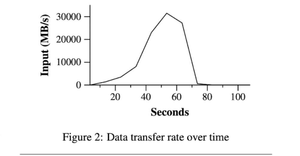
图显示了计算随时间推移的进度。Y 轴显示扫描输入数据的速率。随着更多的机器被分配到这个 MapReduce 计算,速率逐渐回升,当分配了 1764 个 worker 时,速率的峰值超过 30 GB / s。当 map 任务完成时,速率开始下降,并在计算中大约 80 秒处达到零。整个计算从开始到结束大约需要 150 秒。这包括大约一分钟的启动开销。开销是由于程序传播到所有 woker 机器,以及与 GFS 交互以打开 1000 个输入文件集和获取局部性优化所需信息的延迟。
5.3 Sort
排序程序对 1010 条 100-bytes 记录(大约 1TB 的数据)进行排序。该程序以 TeraSort 基准测试为蓝本。
排序程序由少于 50 行的用户代码组成。三行 Map 函数从文本行中提取 10-bytes 排序键,并将该键和原始文本行作为中间键/值对发出。我们使用内置的 identifty 函数作为 reduce 运算符。此函数将中间键/值对作为输出键/值对传递,保持不变。最终的排序输出被写入一组双向复制的 GFS 文件(i.e. 2TB 被写入为程序的输出)。
与之前一样,输入数据被拆分为 64MB 的片段 $(M=15000)$。我们将排序后的输出划分为 4000 个文件 $(R=4000)$。分区函数使用密钥的初始字节将其隔离为 $R$ 的片段之一。
我们针对此基准测试的分区功能内置了密钥分布知识。在常规排序程序中,我们将添加一个 pre-pass MapReduce 操作,该操作将收集键的样本,并使用 samples of the keys 的分布来计算最终排序传递的 split-points。
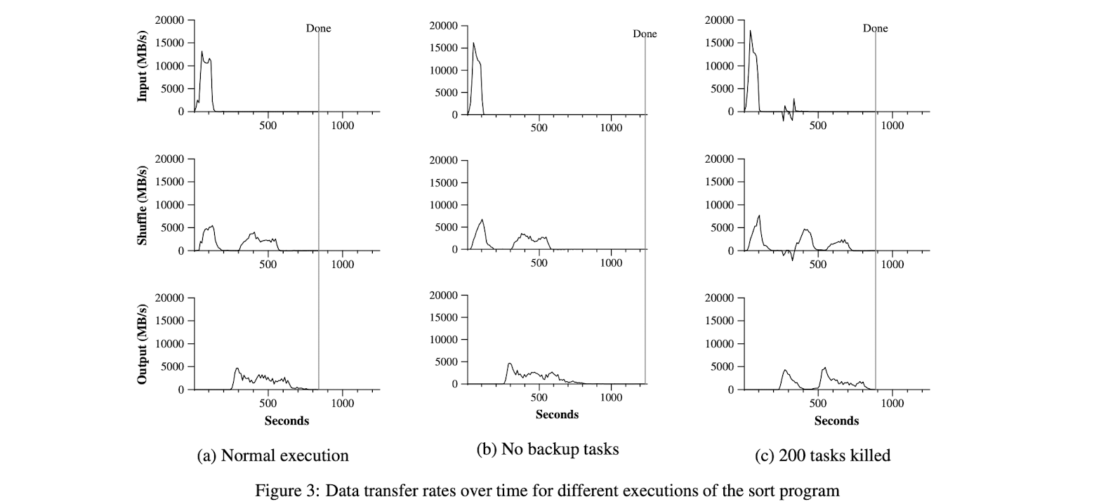
Figure 3 (a) shows the progress of a normal execution of the sort program. The top-left graph shows the rate at which input is read. The rate peaks at about 13 GB/s and dies off fairly quickly since all map tasks finish be- fore 200 seconds have elapsed. Note that the input rate is less than for grep. This is because the sort map tasks spend about half their time and I/O bandwidth writing in- termediate output to their local disks. The corresponding intermediate output for grep had negligible size.
The middle-left graph shows the rate at which data is sent over the network from the map tasks to the re- duce tasks. This shuffling starts as soon as the first map task completes. The first hump in the graph is for the first batch of approximately 1700 reduce tasks (the entire MapReduce was assigned about 1700 machines, and each machine executes at most one reduce task at a time). Roughly 300 seconds into the computation, some of these first batch of reduce tasks finish and we start shuffling data for the remaining reduce tasks. All of the shuffling is done about 600 seconds into the computation.
The bottom-left graph shows the rate at which sorted data is written to the final output files by the reduce tasks. There is a delay between the end of the first shuffling pe- riod and the start of the writing period because the ma- chines are busy sorting the intermediate data. The writes continue at a rate of about 2-4 GB/s for a while. All of the writes finish about 850 seconds into the computation. Including startup overhead, the entire computation takes 891 seconds. This is similar to the current best reported result of 1057 seconds for the TeraSort benchmark [18].
A few things to note: the input rate is higher than the shuffle rate and the output rate because of our locality optimization – most data is read from a local disk and bypasses our relatively bandwidth constrained network. The shuffle rate is higher than the output rate because the output phase writes two copies of the sorted data (we make two replicas of the output for reliability and avail- ability reasons). We write two replicas because that is the mechanism for reliability and availability provided by our underlying file system. Network bandwidth re- quirements for writing data would be reduced if the un- derlying file system used erasure coding [14] rather than replication.
5.4 Effect of Backup Tasks
In Figure 3(b), we show an execution of the sort pro- gram with backup tasks disabled. The execution flow is similar to that shown in Figure 3 (a), except that there is a very long tail where hardly any write activity occurs. After 960 seconds, all except 5 of the reduce tasks are completed. However these last few stragglers don’t fin- ish until 300 seconds later. The entire computation takes 1283 seconds, an increase of 44% in elapsed time.
5.5 Machine Failures
In Figure 3 (c), we show an execution of the sort program where we intentionally killed 200 out of 1746 worker processes several minutes into the computation. The underlying cluster scheduler immediately restarted new worker processes on these machines (since only the pro- cesses were killed, the machines were still functioning properly).
The worker deaths show up as a negative input rate since some previously completed map work disappears (since the corresponding map workers were killed) and needs to be redone. The re-execution of this map work happens relatively quickly. The entire computation fin- ishes in 933 seconds including startup overhead (just an increase of 5% over the normal execution time).
6 Experience
We wrote the first version of the MapReduce library in February of 2003, and made significant enhancements to it in August of 2003, including the locality optimization, dynamic load balancing of task execution across worker machines, etc. Since that time, we have been pleasantly surprised at how broadly applicable the MapReduce li- brary has been for the kinds of problems we work on. It has been used across a wide range of domains within Google, including:
- • large-scale machine learning problems,
- • clustering problems for the Google News and Froogle products,
- • extraction of data used to produce reports of popular queries (e.g. Google Zeitgeist),
- • extractionofpropertiesofwebpagesfornewexper- iments and products (e.g. extraction of geographi- cal locations from a large corpus of web pages for localized search), and
- • large-scale graph computations.
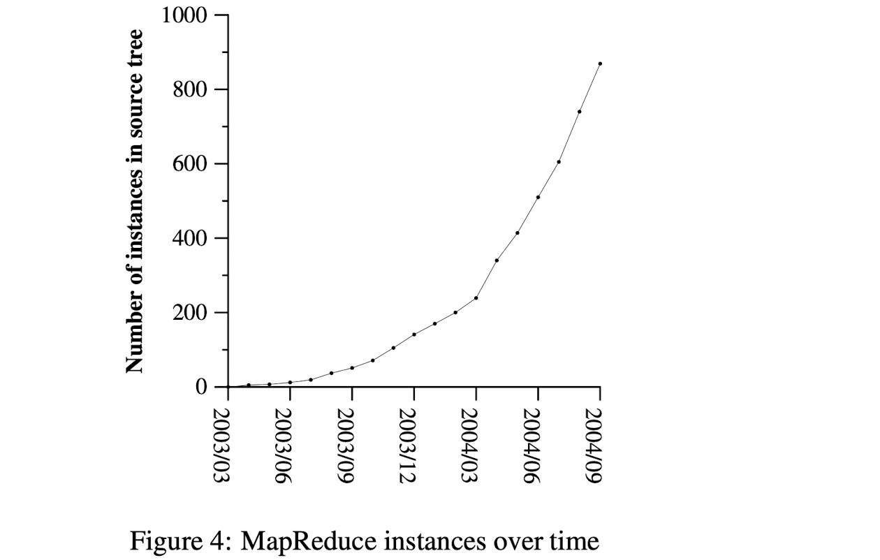
Figure 4 shows the significant growth in the number of separate MapReduce programs checked into our primary source code management system over time, from 0 in early 2003 to almost 900 separate instances as of late September 2004. MapReduce has been so successful be- cause it makes it possible to write a simple program and run it efficiently on a thousand machines in the course of half an hour, greatly speeding up the development and prototyping cycle. Furthermore, it allows programmers who have no experience with distributed and/or parallel systems to exploit large amounts of resources easily.
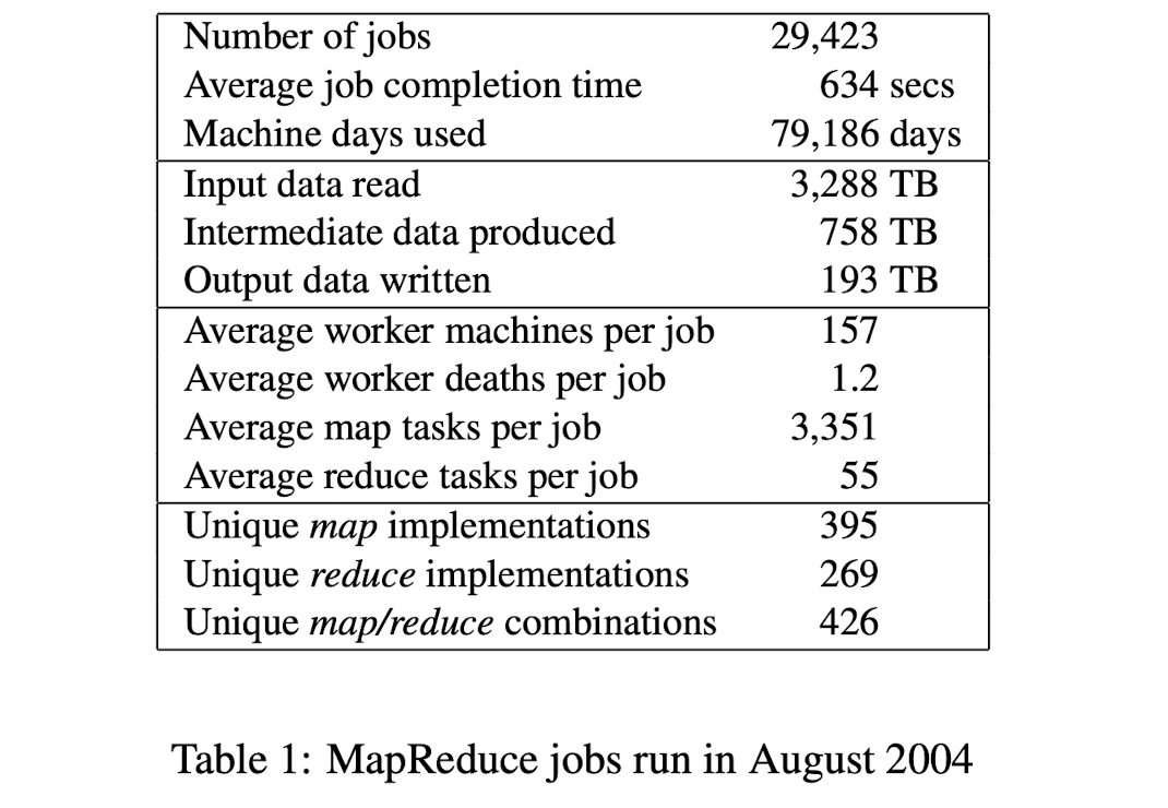
At the end of each job, the MapReduce library logs statistics about the computational resources used by the job. In Table 1, we show some statistics for a subset of MapReduce jobs run at Google in August 2004.
6.1 Large-Scale Indexing
One of our most significant uses of MapReduce to date has been a complete rewrite of the production index-ing system that produces the data structures used for the Google web search service. The indexing system takes as input a large set of documents that have been retrieved by our crawling system, stored as a set of GFS files. The raw contents for these documents are more than 20 ter- abytes of data. The indexing process runs as a sequence of five to ten MapReduce operations. Using MapReduce (instead of the ad-hoc distributed passes in the prior version of the indexing system) has provided several benefits:
- • The indexing code is simpler, smaller, and easier to understand, because the code that deals with fault tolerance, distribution and parallelization is hidden within the MapReduce library. For example, the size of one phase of the computation dropped from approximately 3800 lines of C++ code to approx- imately 700 lines when expressed using MapReduce.
- • The performance of the MapReduce library is good enough that we can keep conceptually unrelated computations separate, instead of mixing them to- gether to avoid extra passes over the data. This makes it easy to change the indexing process. For example, one change that took a few months to make in our old indexing system took only a few days to implement in the new system.
- • The indexing process has become much easier to operate, because most of the problems caused by machine failures, slow machines, and networking hiccups are dealt with automatically by the MapRe- duce library without operator intervention. Further- more, it is easy to improve the performance of the indexing process by adding new machines to the in- dexing cluster.
7 Related Work
Many systems have provided restricted programming models and used the restrictions to parallelize the com- putation automatically. For example, an associative func- tion can be computed over all prefixes of an N element array in log N time on N processors using parallel prefix computations [6, 9, 13]. MapReduce can be considered a simplification and distillation of some of these models based on our experience with large real-world compu- tations. More significantly, we provide a fault-tolerant implementation that scales to thousands of processors. In contrast, most of the parallel processing systems have only been implemented on smaller scales and leave the details of handling machine failures to the programmer.
Bulk Synchronous Programming [17] and some MPI primitives [11] provide higher-level abstractions that make it easier for programmers to write parallel pro- grams. A key difference between these systems and MapReduce is that MapReduce exploits a restricted pro- gramming model to parallelize the user program auto- matically and to provide transparent fault-tolerance.
Our locality optimization draws its inspiration from techniques such as active disks [12, 15], where compu- tation is pushed into processing elements that are close to local disks, to reduce the amount of data sent across I/O subsystems or the network. We run on commodity processors to which a small number of disks are directly connected instead of running directly on disk controller processors, but the general approach is similar.
Our backup task mechanism is similar to the eager scheduling mechanism employed in the Charlotte Sys- tem [3]. One of the shortcomings of simple eager scheduling is that if a given task causes repeated failures, the entire computation fails to complete. We fix some in- stances of this problem with our mechanism for skipping bad records.
The MapReduce implementation relies on an in-house cluster management system that is responsible for dis- tributing and running user tasks on a large collection of shared machines. Though not the focus of this paper, the cluster management system is similar in spirit to other systems such as Condor [16].
The sorting facility that is a part of the MapReduce library is similar in operation to NOW-Sort [1]. Source machines (map workers) partition the data to be sorted and send it to one of R reduce workers. Each reduce worker sorts its data locally (in memory if possible). Of course NOW-Sort does not have the user-definable Map and Reduce functions that make our library widely applicable.
River [2] provides a programming model where pro- cesses communicate with each other by sending data over distributed queues. Like MapReduce, the River system tries to provide good average case performance even in the presence of non-uniformities introduced by heterogeneous hardware or system perturbations. River achieves this by careful scheduling of disk and network transfers to achieve balanced completion times. MapRe- duce has a different approach. By restricting the programming model, the MapReduce framework is able to partition the problem into a large number of fine- grained tasks. These tasks are dynamically scheduled on available workers so that faster workers process more tasks. The restricted programming model also allows us to schedule redundant executions of tasks near the end of the job which greatly reduces completion time in the presence of non-uniformities (such as slow or stuck workers).
BAD-FS [5] has a very different programming model from MapReduce, and unlike MapReduce, is targeted to the execution of jobs across a wide-area network. How- ever, there are two fundamental similarities. (1) Both systems use redundant execution to recover from data loss caused by failures. (2) Both use locality-aware scheduling to reduce the amount of data sent across con- gested network links.
TACC [7] is a system designed to simplify con- struction of highly-available networked services. Like MapReduce, it relies on re-execution as a mechanism for implementing fault-tolerance.
8 Conclusions
The MapReduce programming model has been success- fully used at Google for many different purposes. We attribute this success to several reasons. First, the model is easy to use, even for programmers without experience with parallel and distributed systems, since it hides the details of parallelization, fault-tolerance, locality opti- mization, and load balancing. Second, a large variety of problems are easily expressible as MapReduce com- putations. For example, MapReduce is used for the gen- eration of data for Google’s production web search ser- vice, for sorting, for data mining, for machine learning, and many other systems. Third, we have developed an implementation of MapReduce that scales to large clus- ters of machines comprising thousands of machines. The implementation makes efficient use of these machine re- sources and therefore is suitable for use on many of the large computational problems encountered at Google.
We have learned several things from this work. First, restricting the programming model makes it easy to par- allelize and distribute computations and to make such computations fault-tolerant. Second, network bandwidth is a scarce resource. A number of optimizations in our system are therefore targeted at reducing the amount of data sent across the network: the locality optimization al- lows us to read data from local disks, and writing a single copy of the intermediate data to local disk saves network bandwidth. Third, redundant execution can be used to reduce the impact of slow machines, and to handle ma- chine failures and data loss.
Acknowledgements
Josh Levenberg has been instrumental in revising and extending the user-level MapReduce API with a num- ber of new features based on his experience with using MapReduce and other people’s suggestions for enhance- ments. MapReduce reads its input from and writes its output to the Google File System [8]. We would like to thank Mohit Aron, Howard Gobioff, Markus Gutschke, David Kramer, Shun-Tak Leung, and Josh Redstone for their work in developing GFS. We would also like to thank Percy Liang and Olcan Sercinoglu for their work in developing the cluster management system used by MapReduce. Mike Burrows, Wilson Hsieh, Josh Leven- berg, Sharon Perl, Rob Pike, and Debby Wallach pro- vided helpful comments on earlier drafts of this pa- per. The anonymous OSDI reviewers, and our shepherd, Eric Brewer, provided many useful suggestions of areas where the paper could be improved. Finally, we thank all the users of MapReduce within Google’s engineering or- ganization for providing helpful feedback, suggestions, and bug reports.
Lab
Google File System
Paper
0 ABSTRACT
适用于大型分布式数据密集型应用的可扩展分布式文件系统。它在廉价的商用硬件上运行的同时提供容错能力,并为大量客户端提供高聚合性能。
在本文中,我们介绍了旨在支持分布式应用程序的文件系统接口扩展,讨论了我们设计的许多方面,并报告了微基准测试和实际使用的测量结果。
1 INTRODUCTION
性能、可扩展性、可靠性和可用性。但是,设计对应用程序工作负载和技术环境的关键观察所驱动的,这反映了与一些早期文件系统设计假设的明显背离。
首先,组件故障是常态,而不是例外。
持续监控、错误检测、容错和自动恢复必须成为系统不可或缺的一部分。
其次,按照传统标准,文件很大。
GB 文件很常见。每个文件通常包含许多应用程序对象,如 Web 文档。
当我们经常使用由数十亿个对象组成的许多TB的快速增长的数据集时,即使文件系统可以支持它,管理数十亿个近似KB大小的文件也是笨拙的。
因此,必须重新审视设计假设和参数,如 I/O 操作和块大小。
第三,大多数文件都是通过附加新数据而不是覆盖现有数据来修改的。
文件中的随机写入几乎不存在。写入后,文件仅被读取,并且通常仅按顺序读取。各种数据共享这些特征。
有些可能构成大型存储库,数据分析程序会扫描这些存储库。有些可能是由正在运行的应用程序连续生成的数据流。有些可能是存档数据。有些可能是在一台机器上产生并在另一台机器上处理的中间结果,无论是同时还是稍后。
鉴于这种对大型文件的访问模式,追加成为性能优化和原子性保证的重点,而在客户端中缓存数据块则失去了吸引力。
第四,应用程序和文件系统API的协同设计提高了整个系统的灵活性。例如:
我们放宽了 GFS 的一致性模型 consistency model 要求,以大大简化 GFS 设计,而不会给应用程序带来沉重的负担。
我们还引入了原子的记录追加操作,以便多个客户端可以并发追加到一个文件,不需要额外的同步操作来保证数据的一致性。
2 DESIGN OVERVIEW
2.1 Assumptions
我们之前提到了一些关键的观察结果,现在更详细地阐述了我们的假设。
- 系统必须持续监控自身的状态,它必须将组件失效作为一种常态,能够迅速地侦测、冗余并恢复失效的组件。
- 系统存储适量的大文件,预计会有几百万个文件,每个文件的大小通常为 100MB 或更大。GB 级别的文件也很常见,应进行有效管理。GFS 也必须支持小文件,但不需要针对它们进行优化。
- 工作负载主要由两种读取组成:大型流式读取和小型随机读取。
- 在大型流式读取中,单个操作通常读取数百 KB,更常见的是 1MB 或更多。来自同一客户端的连续操作通常会读取文件的连续区域。
- 小规模的随机读取通常是在文件某个随机的位置读取几个 KB 数据。如果应用程序对性能非常关注,通常的做法是把小规模的随机读取操作合并并排序,之后按顺序批量读取,以在文件中稳步前进,而避免在文件中前后来回的移动读取位置。
- 系统的工作负载还包括许多大规模的、顺序的、数据追加方式的写操作。典型的操作大小与读取操作的大小类似。写入后,文件很少会再次修改。GFS 支持在文件中任意位置进行小规模的随机写入操作,但是可能效率不彰。
- 系统必须高效的、行为定义明确的(alex注:well-defined)实现多客户端并行追加数据到同一个文件里的语意。我们的文件通常被用于“生产者-消费者”队列,或者其它多路文件合并操作。数百个生产者,每台计算机运行一个生产者,将同时对一个文件进行 append 操作。使用最小的同步开销来实现的原子的多路追加数据操作是必不可少的。文件可稍后读取,或者是消费者在追加的操作的同时读取文件。
- 高性能的稳定网络带宽远比低延迟重要。我们的目标程序绝大部分要求能够高速率的、大批量的处理 数据,极少有程序对单一的读写操作有严格的响应时间要求。
2.2 Interface
GFS 提供了一套不是严格按照 POSIX 等标准 API 的形式实现的类似传统文件系统的 API 接口函数。文件以分层目录的形式组织,用路径名来标识,支持常用的操作,如创建新文件、删除文件、打开文件、关闭文件、读和写文件。
此外,GFS 还具有快照和记录追加操作。
- 快照以低成本创建文件或目录树的副本。
- 记录追加允许多个客户端并发对同一文件进行 append 操作,同时保证每个客户端追加操作的原子性。
它对于实现多路合并结果和“生产者-消费者”队列非常有用 —— 多个客户端可以在不需要额外的同步锁定的情况下,同时对一个文件追加数据。
我们发现这些类型的文件对于构建大型分布应用是非常重要的。
2.3 Architecture
GFS 集群包含单个 $master$ 节点、多个 $chunkservers$ 组成,并同时由多个 $clients$ 访问,如图 1 所示。
所有机器通常都是运行着 user-level 服务进程的普通 Linux machine。只要机器资源允许,可以很容易的把 $chunkserver$ 和 $client$ 都放在同一台机器上运行,并且我们能够接受不可靠的应用程序代码带来的稳定性降低的风险。

GFS 存储文件被划分为固定大小的 $chunks$。
- 每个 $chunk$ 创建时都由 $master$ 分配一个不变、全局唯一的 $64\ bit\ chunks\ handle$ 标识。
- $chunkservers$ 将 $chunks$ 以 Linux 文件形式存储在本地磁盘,并根据指定的 $chunk\ handle$ 和 $byte\ range$ 读写块数据。为提高可靠性,每个 $chunk$ 都会被复制到多个 $chunkservers$ 上。
- 默认情况下,我们使用 3 个存储复制节点,但用户可以为不同的文件命名空间设定不同的复制级别。
master 节点管理所有文件系统的元数据。这包含
- $the\ namespace$,
- $access\ control\ information$,
- $the\ mapping\ from\ files\ to\ chunks$,
- $the\ current\ locations\ of\ chunks$
master 节点管理系统范围的活动,例如
- $chunk\ lease\ management$,
- $garbage\ collection\ of\ orphaned\ chunks$,
- $chunk\ migration\ between\ chunkservers$
$master$ 节点使用 $HeartBeat\ message$ 周期性地和每个 $chunkserver$ 通信,发送指令到各个 $chunkservers$ 并接收 $chunkservers$ 的状态信息。
GFS $clients$ 代码以 $library$ 的形式被链接到客户程序里。
- 客户端代码实现了 GFS 文件系统的 API 接口函数、应用程序与 $master$ 节点和 $chunkserver$ 通讯、以及对数据进行读写操作。
- 客户端和 $master$ 节点的通信只获取元数据,所有的数据操作都是由客户端直接和 $chunkserver$ 进行交互的。
- 我们不提供 POSIX 标准的 API 的功能,因此,GFS API 调用不需要深入到Linux vnode级别。
客户端和 $chunkserver$ 都不需要缓存文件数据。
- 客户端缓存几乎无用(但是,客户端会缓存元数据),因为大部分程序要么以流的方式读取巨大文件,要么工作集太大无法被缓存。无需考虑缓存相关问题可以通过消除缓存一致性问题来简化客户端和整个系统的实现。
- $chunkservers$ 不需要缓存文件数据,因为 $chunks$ 以本地文件方式存储,Linux 的文件系统缓存会把经常访问的数据缓存在内存中。
2.4 Single Master
单一 $master$ 节点策略大大简化了 GFS 设计
- 单一的 $master$ 节点可以通过全局的信息精确定位 $chunks$ 的位置以及进行复制决策。
- 但是,我们须减少它对 $master$ 节点的读写,以免 $master$ 节点成为系统瓶颈。
客户端从不通过 $master$ 节点读写文件数据。相反,客户端会询问 $master$ 节点它应该联系哪些 $chunkserver$。它将此信息缓存一段 certain 时间,后续的操作将直接和 $chunkserver$ 进行数据读写操作。
参考图 1 简单解释一次简单读取的流程。
首先,客户端根据固定的 Chunk size,把文件名和程序指定的字节偏移 [转换] 成文件的 chunk index 。
然后,它把文件名和 chunk index 发送给 $master$ 节点。$master$ 节点将相应的 chunk handle 和副本的位置信息回复给客户端。客户端用文件名和 chunk index 作为 key 缓存这些 信息。
然后,客户端向其中一个副本(很可能是最近的副本)发送请求。请求信息包含了 $chunks\ handler$ 标识和字节范围。在对这个 $chunks$ 的后续读取操作中,客户端不必再和 $master$ 节点通讯了,除非缓存的元数据信息过期或者文件被重新打开。
实际上,客户端通常在同一请求中请求多个 $chunks$ 信息, $master$ 节点的回应也可能包含了紧跟着这些被请求的 $chunks$ 后面的 $chunks$ 的信息。实际中,这些额外的信息避免了客户端和 $master$ 节点未来可能会发生的几次通讯,而几乎不需要额外的成本。
2.5 Chunk Size
Chunk size 是关键设计参数之一。我们选择了 64MB,远大于一般文件系统的 Block size。每个 $chunks$ 的副本都作为普通 Linux 文件存储在 $chunkserver$ 上,仅在需要时进行扩展。惰性空间分配策略避免了由于内部碎片导致的空间浪费,这可能是对 suck a large chunk size 的最大争议。
Large $chunk$ size 提供了几个重要的优点。
- 首先,它减少了客户端和 $master$ 节点通讯的需求,因为仅需一次和 $master$ 节点的通信,就可以获取 $chunk$ 的位置信息,之后就可以对同一个 $chunk$ 进行多次的读写操作。这种方式对降低我们的工作负载来说效果显著,因为我们的应用程序通常是连续读写大文件。即使是小规模的随机读取,采用较大的 $chunk$ 尺寸也带来明显的好处,客户端可以轻松的缓存一个数TB的工作数据集所有的 $chunk$ 位置信息。
- 其次,采用较大的 $chunk$ 尺寸,客户端能够对一个块进行多次操作,这样就可以通过与 $chunk$ 服务器保持较长时间的 TCP 连接来减少网络负载。
- 第三,选用较大的 $chunk$ 尺寸减少了 $master$ 节点需要保存的元数据的数量。这就允许我们把元数据全部放在内存中,在2.6.1节我们会讨论元数据全部放在内存中带来的额外的好处。
另一方面,即使有惰性空间分配,大的 $chunk\ size$ 也有其缺点:一个小文件包含较少的 $chunk$ ,甚至仅一个。当有许多的客户端对同一个小文件进行多次的访问时,存储这些 $chunk$ 的 $chunk\ server$ 会变成热点。
在实际应用中,由于我们的程序通常是连续的读取包含多个 $chunk$ 的大文件,热点还不是主要的问题。
然而,当我们第一次把 GFS 用于批处理队列系统的时候,热点的问题还是产生了:一个可执行文件在 GFS 上保存为 $single-chunk$ 文件,之后这个可执行文件在数百台机器上同时启动。存放这个可执行文件的几个 $chunk\ server$ 被数百个客户端的并发请求访问导致系统局部过载。|我们通过使用更大的复制参数来保存可执行文件,以及错开批处理队列系统程序的启动时间的方法解决了这个问题。
一个可能的长效解决方案是,在这种的情况下,允许客户端从其它客户端读取数据。
2.6 Metadata
$master$ 节点存储三种主要类型的元数据:
alex注:注意逻辑的 $master$ 节点和物理的 $master server$ 的区别。后续我们谈的是每个 $master server$ 的行为,如存储、内存等等,因此我们将全部使用物理名称
- 文件和 $chunk$ 的命名空间
- 从文件到 $chunk$ 的映射关系
- 以及每个 $chunk$ 副本的存储位置
所有元数据都保存在 $master server$ 的内存中。
- 前两种类型的元数据 (namespaces & file-to-chunkmapping) 同时也会以记录变更日志的方式记录在操作系统的系统日志文件中,日志文件存储在本地磁盘上,同时日志会被复制到其它的远程 $master server$ 上。
采用保存变更日志的方式,我们能够简单可靠的更新 $master server$ 的状态,并且不用担心 $master server$ 崩溃导致数据不一致的风险。 $master server$ 不会持久保存 $chunk$ 位置信息。 $master server$ 在启动时,或者有新的 $chunk\ server$ 加入时,向各个 $master server$ 轮询它们所存储的 $chunk$ 的信息。
2.6.1 In-Memory Data Structures
因为元数据保存在内存中,所以Master服务器的操作速度非常快。并且,Master服务器可以在后台简单而高效的周期性扫描自己保存的全部状态信息。这种周期性的状态扫描也用于实现Chunk垃圾收集、在Chunk服务器失效的时重新复制数据、通过Chunk的迁移实现跨Chunk服务器的负载均衡以及磁盘使用状况统计等功能。(4.3 & 4.4深入讨论)
将元数据全部保存在内存中的方法有潜在问题:
- Chunk的数量以及整个系统的承载能力都受限于Master服务器所拥有的内存大小。
- 但在实际应用中,这并不是一个严重的问题。
- Master服务器只需要不到 64 个字节的元数据就能够管理一个 64MB 的 $chunk$ 。由于大多数文件都包含多个 $chunk$ ,因此绝大多数 $chunk$ 都是满的,除了文件的最后一个 $chunk$ 是部分填充的。同样的,每个文件的在命名空间中的数据大小通常在 64 字节以下,因为保存的文件名是用前缀压缩算法压缩过的。
即便是需要支持更大的文件系统,为Master服务器增加额外内存的费用是很少的,而通过增加有限的费用,我们就能够把元数据全部保存在内存里,增强了系统的简洁性、可靠性、高性能和灵活性。
2.6.2 Chunk Locations
Master服务器并不持久化保存哪个Chunk服务器存有指定Chunk的副本的信息。Master服务器仅在启动的时候轮询Chunk服务器以获取这些信息。Master服务器能够保证它持有的信息始终是最新的,因为它控制了所有的Chunk位置的分配,而且通过周期性的 $Heartbeat\ Message$ 监控Chunk服务器的状态。
最初设计时,我们试图把Chunk的位置信息持久的保存在Master服务器上,但是后来我们发现在启动的时候轮询Chunk服务器,之后定期轮询更新的方式更简单。这种设计简化了在有Chunk服务器加入集群、离开集群、更名、失效、以及重启的时候,Master服务器和Chunk服务器数据同步的问题。在一个拥有数百台服务器的集群中,这类事件会频繁的发生。
可以从另外一个角度去理解这个设计决策:只有Chunk服务器才能最终确定一个Chunk是否在它的硬盘上。
我们从没有考虑过在Master服务器上维护一个这些信息的全局视图,因为Chunk服务器的错误可能会导致Chunk自动消失(比如,硬盘损坏了或者无法访问了),亦或者操作人员可能会重命名一个Chunk服务器。
2.6.3 Operation Log
操作日志包含了关键的元数据变更历史记录。对 GFS 非常重要。
操作日志是元数据唯一的持久化存储记录
也作为判断同步操作顺序的逻辑时间基线
alex注:也就是通过逻辑日志的序号作为操作发生的逻辑时间,类似于事务系统中的 LSN
文件和Chunk,连同它们的版本(参考4.5节),都由它们创建的逻辑时间唯一的、永久的标识。
必须确保日志文件的完整,确保只有在元数据的变化被持久化后,日志才对客户端是可见的。否则,即使Chunk本身没有出现任何问题,我们仍有可能丢失整个文件系统,或者丢失客户端最近的操作。所以,我们会把日志复制到多台远程机器,并且只有把相应的日志记录写入到本地以及远程机器的硬盘后,才会响应客户端的操作请求。Master服务器会收集多个日志记录后批量处理,以减少写入磁盘和复制对系统整体性能的影响。
Master服务器在灾难恢复时,通过重演操作日志把文件系统恢复到最近的状态。为了缩短Master启动的时间,我们必须使日志足够小。(alex注:即重演系统操作的日志量尽量的少)
Master服务器在日志增长到一定量时对系统状态做一次Checkpoint(alex注:Checkpoint是一种行为,一种对数据库状态作一次快照的行为),将所有的状态数据写入一个Checkpoint文件(alex注:并删除之前的日志文件)。在灾难恢复的时候,Master服务器就通过从磁盘上读取这个Checkpoint文件,以及重演Checkpoint之后的有限个日志文件就能够恢复系统。Checkpoint 文件以压缩B-树形式的数据结构存储,可以直接映射到内存,在用于命名空间查询时无需额外的解析。这大大提高了恢复速度,增强了可用性。
由于创建一个Checkpoint文件需要一定的时间,所以Master服务器的内部状态被组织为一种格式,这种格式要确保在Checkpoint过程中不会阻塞正在进行的修改操作。Master服务器使用独立的线程切换到新的日志文件和创建新的Checkpoint文件。新的Checkpoint文件包括切换前所有的修改。对于一个包含数百万个文件的集群,创建一个Checkpoint文件需要1分钟左右的时间。创建完成后,Checkpoint文件会被写入在本地和远程的硬盘里。
Master服务器恢复只需要最新的Checkpoint文件和后续的日志文件。旧的Checkpoint文件和日志文件可以被删除,但是为了应对灾难性的故障 (alex注:catastrophes,数据备份相关文档中经常会遇到这个词,表示一种超出预期范围的灾难性事件),我们通常会多保存一些历史文件。Checkpoint失败不会对正确性产生任何影响,因为恢复功能的代码可以检测并跳过没有完成的Checkpoint文件。
2.7 Consistency Model
GFS 支持一个宽松的一致性模型,这个模型能够很好的支撑我们的高度分布的应用,同时还保持了相对简单且容易实现的优点。本节我们讨论 GFS 的一致性的保障机制,以及对应用程序的意义。我们也着重描述了GFS如何管理这些一致性保障机制,但是实现的细节将在本论文的其它部分讨论。
2.7.1 Guarantees by GFS
文件命名空间的修改(例如,文件创建)是原子性的。它们仅由Master节点的控制:
- 命名空间锁提供了原子性和正确性(4.1章)的保障;
- Master节点的操作日志定义了这些操作在全局的顺序(2.6.3章)。
数据修改后文件region的状态取决于操作的类型、成功与否、以及是否同步修改。表1总结了各种操作的结果。
alex注:region这个词用中文非常难以表达,我认为应该是修改操作所涉及的文件中的某个范围

如果所有客户端,无论从哪个副本读取,读到的数据都一样,那么我们认为文件region是“一致的”;如果对文件的数据修改之后,region是一致的,并且客户端能够看到写入操作全部的内容,那么这个region是“已定义的”。当一个数据修改操作成功执行,并且没有受到同时执行的其它写入操作的干扰,那么影响的region就是已定义的(隐含了一致性):所有的客户端都可以看到写入的内容。并行修改操作成功完成之后,region处于一致的、未定义的状态:所有的客户端看到同样的数据,但是无法读到任何一次写入操作写入的数据。通常情况下,文件region内包含了来自多个修改操作的、混杂的数据片段。失败的修改操作导致一个region处于不一致状态(同时也是未定义的):不同的客户在不同的时间会看到不同的数据。后面我们将描述应用如何区分已定义和未定义的region。应用程序没有必要再去细分未定义region的不同类型。
数据修改操作分为写入或者记录追加两种。写入操作把数据写在应用程序指定的文件偏移位置上。即使有多个修改操作并行执行时,记录追加操作至少可以把数据原子性的追加到文件中一次,但是偏移位置是由GFS选择的(3.3章)。(相比而言,通常说的追加操作写的偏移位置是文件的尾部。)
(alex注:这句话有点费解,其含义是所有的追加写入都会成功,但是有可能被执行了多次,而且每次追加的文件偏移量由GFS自己计算)
GFS返回给客户端一个偏移量,表示了包含了写入记录的、已定义的region的起点。另外,GFS可能会在文件中间插入填充数据或者重复记录。这些数据占据的文件region被认定是不一致的,这些数据通常比用户数据小的多。
经过了一系列的成功的修改操作之后,GFS确保被修改的文件region是已定义的,并且包含最后一次修改操作写入的数据。GFS通过以下措施确保上述行为:
(a)对Chunk的所有副本的修改操作顺序一致(3.1章),
(b)使用Chunk的版本号来检测副本是否因为它所在的Chunk服务器宕机(4.5章)而错过了修改操作而导致其失效。失效的副本不会再进行任何修改操作,Master服务器也不再返回这个Chunk副本的位置信息给客户端。它们会被垃圾收集系统尽快回收。
由于Chunk位置信息会被客户端缓存,所以在信息刷新前,客户端有可能从一个失效的副本读取了数据。在缓存的超时时间和文件下一次被打开的时间之间存在一个时间窗,文件再次被打开后会清除缓存中与该文件有关的所有Chunk位置信息。而且,由于我们的文件大多数都是只进行追加操作的,所以,一个失效的副本通常返回一个提前结束的Chunk而不是过期的数据。当一个Reader重新尝试并联络Master服务器时,它就会立刻得到最新的Chunk位置信息。
(alex注:本文中将用到两个专有名词,Reader和Writer,分别表示执行GFS读取和写入操作的程序)
即使在修改操作成功执行很长时间之后,组件的失效也可能损坏或者删除数据。GFS通过Master服务器和所有Chunk服务器的定期“握手”来找到失效的Chunk服务器,并且使用Checksum来校验数据是否损坏(5.2章)。一旦发现问题,数据要尽快利用有效的副本进行恢复(4.3章)。只有当一个Chunk的所有副本在GFS检测到错误并采取应对措施之前全部丢失,这个Chunk才会不可逆转的丢失。在一般情况下GFS的反应时间(alex注:指Master节点检测到错误并采取应对措施)是几分钟。即使在这种情况下,Chunk也只是不可用了,而不是损坏了:应用程序会收到明确的错误信息而不是损坏的数据。
2.7.2 Implications for Applications
使用GFS的应用程序可以利用一些简单技术实现这个宽松的一致性模型,这些技术也用来实现一些其它的
目标功能,包括:尽量采用追加写入而不是覆盖,Checkpoint,自验证的写入操作,自标识的记录。
在实际应用中,我们所有的应用程序对文件的写入操作都是尽量采用数据追加方式,而不是覆盖方式。一种典型的应用,应用程序从头到尾写入数据,生成了一个文件。写入所有数据之后,应用程序自动将文件改名为一个永久保存的文件名,或者周期性的作Checkpoint,记录成功写入了多少数据。Checkpoint文件可以包含程序级别的校验和。Readers仅校验并处理上个Checkpoint之后产生的文件region,这些文件region的状态一定是已定义的。这个方法满足了我们一致性和并发处理的要求。追加写入比随机位置写入更加有效率,对应用程序的失败处理更具有弹性。Checkpoint可以让Writer以渐进的方式重新开始,并且可以防止Reader处理已经被成功写入,但是从应用程序的角度来看还并未完成的数据。
我们再来分析另一种典型的应用。许多应用程序并行的追加数据到同一个文件,比如进行结果的合并或者是一个生产者-消费者队列。记录追加方式的“至少一次追加”的特性保证了Writer的输出。Readers使用下面的方法来处理偶然性的填充数据和重复内容。Writers在每条写入的记录中都包含了额外的信息,例如Checksum,用来验证它的有效性。Reader可以利用Checksum识别和抛弃额外的填充数据和记录片段。如果应用不能容忍偶尔的重复内容(比如,如果这些重复数据触发了非幂等操作),可以用记录的唯一标识符来过滤它们,这些唯一标识符通常用于命名程序中处理的实体对象,例如web文档。这些记录I/O功能(alex注:ThesefunctionalitiesforrecordI/O)(除了剔除重复数据)都包含在我们的程序共享的库中,并且适用于Google内部的其它的文件接口实现。所以,相同序列的记录,加上一些偶尔出现的重复数据,都被分发到Reader了。
3 SYSTEM INTERACTIONS
我们在设计这个系统时,一个重要的原则是最小化所有操作和Master节点的交互。带着这样的设计理念,我们现在描述一下客户机、Master服务器和Chunk服务器如何进行交互,以实现数据修改操作、原子的记录追加操作以及快照功能。
3.1 Leases and Mutation Order
变更是一个会改变Chunk内容或者元数据的操作,比如写入操作或者记录追加操作。变更操作会在Chunk的所有副本上执行。我们使用租约(lease)机制来保持多个副本间变更顺序的一致性。Master节点为Chunk的一个副本建立一个租约,我们把这个副本叫做主Chunk。主Chunk对Chunk的所有更改操作进行序列化。所有的副本都遵从这个序列进行修改操作。因此,修改操作全局的顺序首先由Master节点选择的租约的顺序决定,然后由租约中主Chunk分配的序列号决定。
设计租约机制的目的是为了最小化Master节点的管理负担。租约的初始超时设置为60秒。不过,只要Chunk被修改了,主Chunk就可以申请更长的租期,通常会得到Master节点的确认并收到租约延长的时间。这些租约延长请求和批准的信息通常都是附加在Master节点和Chunk服务器之间的心跳消息中来传递。有时Master节点会试图提前取消租约(例如,Master节点想取消在一个已经被改名的文件上的修改操作)。即使Master节点和主Chunk失去联系,它仍然可以安全地在旧的租约到期后和另外一个Chunk副本签订新的租约。

在图2中,我们依据步骤编号,展现写入操作的控制流程。
- 客户机向Master节点询问哪一个Chunk服务器持有当前的租约,以及其它副本的位置。如果没有一个Chunk持有租约,Master节点就选择其中一个副本建立一个租约(这个步骤在图上没有显示)。
- Master节点将主Chunk的标识符以及其它副本(又称为secondary副本、二级副本)的位置返回给客户机。客户机缓存这些数据以便后续的操作。只有在主Chunk不可用,或者主Chunk回复信息表明它已不再持有租约的时候,客户机才需要重新跟Master节点联系。
- 客户机把数据推送到所有的副本上。客户机可以以任意的顺序推送数据。Chunk服务器接收到数据并保存在它的内部LRU缓存中,一直到数据被使用或者过期交换出去。由于数据流的网络传输负载非常高,通过分离数据流和控制流,我们可以基于网络拓扑情况对数据流进行规划,提高系统性能,而不用去理会哪个Chunk服务器保存了主Chunk。3.2章节会进一步讨论这点。
- 当所有的副本都确认接收到了数据,客户机发送写请求到主Chunk服务器。这个请求标识了早前推送到所有副本的数据。主Chunk为接收到的所有操作分配连续的序列号,这些操作可能来自不同的客户机,序列号保证了操作顺序执行。它以序列号的顺序把操作应用到它自己的本地状态中(alex注:也就是在本地执行这些操作,这句话按字面翻译有点费解,也许应该翻译为“它顺序执行这些操作,并更新自己的状态”)。
- 主Chunk把写请求传递到所有的二级副本。每个二级副本依照主Chunk分配的序列号以相同的顺序
执行这些操作。 - 所有的二级副本回复主Chunk,它们已经完成了操作。
- 主Chunk服务器(alex注:即主Chunk所在的Chunk服务器)回复客户机。任何副本产生的任何错
误都会返回给客户机。在出现错误的情况下,写入操作可能在主Chu nk和一些二级副本执行成功。(如果操作在主Chunk上失败了,操作就不会被分配序列号,也不会被传递。)客户端的请求被确认为失败,被修改的region处于不一致的状态。我们的客户机代码通过重复执行失败的操作来处理这样的错误。在从头开始重复执行之前,客户机会先从步骤(3)到步骤(7)做几次尝试。
如果应用程序一次写入的数据量很大,或者数据跨越了多个Chunk,GFS客户机代码会把它们分成多个写操作。这些操作都遵循前面描述的控制流程,但是可能会被其它客户机上同时进行的操作打断或者覆盖。因此,共享的文件region的尾部可能包含来自不同客户机的数据片段,尽管如此,由于这些分解后的写入操作在所有的副本上都以相同的顺序执行完成,Chunk的所有副本都是一致的。这使文件region处于2.7节描述的一致的、但是未定义的状态。
3.2 Data Flow
为了提高网络效率,我们采取了把数据流和控制流分开的措施。在控制流从客户机到主Chunk、然后再到所有二级副本的同时,数据以管道的方式,顺序的沿着一个精心选择的Chunk服务器链推送。我们的目标是充分利用每台机器的带宽,避免网络瓶颈和高延时的连接,最小化推送所有数据的延时。
为了充分利用每台机器的带宽,数据沿着一个Chunk服务器链顺序的推送,而不是以其它拓扑形式分散推送(例如,树型拓扑结构)。线性推送模式下,每台机器所有的出口带宽都用于以最快的速度传输数据,而不是在多个接受者之间分配带宽。
为了尽可能的避免出现网络瓶颈和高延迟的链接(eg,inter-switch最有可能出现类似问题),每台机器都尽量的在网络拓扑中选择一台还没有接收到数据的、离自己最近的机器作为目标推送数据。假设客户机把数据从Chunk服务器S1推送到S4。它把数据推送到最近的Chunk服务器S1。S1把数据推送到S2,因为S2和S4中最接近的机器是S2。同样的,S2把数据传递给S3和S4之间更近的机器,依次类推推送下去。我们的网络拓扑非常简单,通过IP地址就可以计算出节点的“距离”。
最后,我们利用基于TCP连接的、管道式数据推送方式来最小化延迟。Chunk服务器接收到数据后,马上开始向前推送。管道方式的数据推送对我们帮助很大,因为我们采用全双工的交换网络。接收到数据后立刻向前推送不会降低接收的速度。在没有网络拥塞的情况下,传送B字节的数据到R个副本的理想时间是B/T+RL,T是网络的吞吐量,L是在两台机器数据传输的延迟。通常情况下,我们的网络连接速度是100Mbps(T),L将远小于1ms。因此,1MB的数据在理想情况下80ms左右就能分发出去。
3.3 Atomic Record Appends
GFS提供了一种原子的数据追加操作–记录追加。传统方式的写入操作,客户程序会指定数据写入的偏移量。对同一个region的并行写入操作不是串行的:region尾部可能会包含多个不同客户机写入的数据片段。使用记录追加,客户机只需要指定要写入的数据。GFS保证至少有一次原子的写入操作成功执行(即写入一个顺序的byte流),写入的数据追加到GFS指定的偏移位置上,之后GFS返回这个偏移量给客户机。这类似于在Unix操作系统编程环境中,对以O_APPEND模式打开的文件,多个并发写操作在没有竞态条件时的行为。
记录追加在我们的分布应用中非常频繁的使用,在这些分布式应用中,通常有很多的客户机并行地对同一个文件追加写入数据。如果我们采用传统方式的文件写入操作,客户机需要额外的复杂、昂贵的同步机制,例如使用一个分布式的锁管理器。在我们的工作中,这样的文件通常用于多个生产者/单一消费者的队列系统,或者是合并了来自多个客户机的数据的结果文件。
记录追加是一种修改操作,它也遵循3.1节描述的控制流程,除了在主Chunk有些额外的控制逻辑。客户机把数据推送给文件最后一个Chunk的所有副本,之后发送请求给主Chunk。主Chunk会检查这次记录追加操作是否会使Chunk超过最大尺寸(64MB)。如果超过了最大尺寸,主Chunk首先将当前Chunk填充到最大尺寸,之后通知所有二级副本做同样的操作,然后回复客户机要求其对下一个Chunk重新进行记录追加操作。(记录追加的数据大小严格控制在Chunk最大尺寸的1/4,这样即使在最坏情况下,数据碎片的数量仍然在可控的范围。)通常情况下追加的记录不超过Chunk的最大尺寸,主Chunk把数据追加到自己的副本内,然后通知二级副本把数据写在跟主Chunk一样的位置上,最后回复客户机操作成功。
如果记录追加操作在任何一个副本上失败了,客户端就需要重新进行操作。重新进行记录追加的结果是,同一个Chunk的不同副本可能包含不同的数据–重复包含一个记录全部或者部分的数据。GFS并不保证Chunk的所有副本在字节级别是完全一致的。它只保证数据作为一个整体原子的被至少写入一次。这个特性可以通过简单观察推导出来:如果操作成功执行,数据一定已经写入到Chunk的所有副本的相同偏移位置上。这之后,所有的副本至少都到了记录尾部的长度,任何后续的记录都会追加到更大的偏移地址,或者是不同的Chunk上,即使其它的Chunk副本被Master节点选为了主Chunk。就我们的一致性保障模型而言,记录追加操作成功写入数据的region是已定义的(因此也是一致的),反之则是不一致的(因此也就是未定义的)。正如我们在2.7.2节讨论的,我们的程序可以处理不一致的区域。
3.4 Snapshot
(alex注:这一节非常难以理解,总的来说依次讲述了什么是快照、快照使用的COW技术、快照如何不干扰当前操作)
快照操作几乎可以瞬间完成对一个文件或者目录树(“源”)做一个拷贝,并且几乎不会对正在进行的其它操作造成任何干扰。我们的用户可以使用快照迅速的创建一个巨大的数据集的分支拷贝(而且经常是递归的拷贝拷贝),或者是在做实验性的数据操作之前,使用快照操作备份当前状态,这样之后就可以轻松的提交或者回滚到备份时的状态。
就像AFS(alex注:AFS,即AndrewFileSystem,一种分布式文件系统),我们用标准的copy-on-write技术实现快照。当Master节点收到一个快照请求,它首先取消作快照的文件的所有Chunk的租约。这个措施保证了后续对这些Chunk的写操作都必须与Master交互交互以找到租约持有者。这就给Master节点一个率先创建Chunk的新拷贝的机会。
租约取消或者过期之后,Master节点把这个操作以日志的方式记录到硬盘上。然后,Master节点通过复制源文件或者目录的元数据的方式,把这条日志记录的变化反映到保存在内存的状态中。新创建的快照文件和源文件指向完全相同的Chunk地址。
在快照操作之后,当客户机第一次想写入数据到ChunkC,它首先会发送一个请求到Master节点查询当前的租约持有者。Master节点注意到ChunkeC的引用计数超过了1(alex注:不太明白为什么会大于1.难道是Snapshot没有释放引用计数?)。Master节点不会马上回复客户机的请求,而是选择一个新的Chunk句柄C。之后,Master节点要求每个拥有ChunkC当前副本的Chunk服务器创建一个叫做C的新Chunk。通过在源Chunk所在Chunk服务器上创建新的Chunk,我们确保数据在本地而不是通过网络复制(我们的硬盘比我们的100Mb以太网大约快3倍)。从这点来讲,请求的处理方式和任何其它Chunk没什么不同:Master节点确保新ChunkC`的一个副本拥有租约,之后回复客户机,客户机得到回复后就可以正常的写这个Chunk,而不必理会它是从一个已存在的Chunk克隆出来的。
4 MASTER OPERATION
The master executes all namespace operations. In addition, it manages chunk replicas throughout the system: it makes placement decisions, creates new chunks and hence replicas, and coordinates various system-wide activities to keep chunks fully replicated, to balance load across all the chunkservers, and to reclaim unused storage. We now discuss each of these topics.
4.1 Namespace Management and Locking
Many master operations can take a long time: for example, a snapshot operation has to revoke chunkserver leases on all chunks covered by the snapshot. We do not want to delay other master operations while they are running. Therefore, we allow multiple operations to be active and use locks over regions of the namespace to ensure proper serialization.
Unlike many traditional file systems, GFS does not have a per-directory data structure that lists all the files in that directory. Nor does it support aliases for the same file or directory (i.e, hard or symbolic links in Unix terms). GFS logically represents its namespace as a lookup table mapping full pathnames to metadata. With prefix compression, this table can be efficiently represented in memory. Each node in the namespace tree (either an absolute file name or an absolute directory name) has an associated read-write lock.
Each master operation acquires a set of locks before it runs. Typically, if it involves /d1/d2/…/dn/leaf, it will acquire read-locks on the directory names /d1, /d1/d2, …, /d1/d2/…/dn, and either a read lock or a write lock on the full pathname /d1/d2/…/dn/leaf. Note that leaf may be a file or directory depending on the operation.
We now illustrate how this locking mechanism can prevent a file /home/user/foo from being created while /home/user is being snapshotted to /save/user. The snapshot operation acquires read locks on /home and /save, and write locks on /home/user and /save/user. The file creation acquires read locks on /home and /home/user, and a write lock on /home/user/foo. The two operations will be serialized properly because they try to obtain conflicting locks on /home/user. File creation does not require a write lock on the parent directory because there is no “directory”, or inode-like, data structure to be protected from modification. The read lock on the name is sufficient to protect the parent directory from deletion.
One nice property of this locking scheme is that it allows concurrent mutations in the same directory. For example, multiple file creations can be executed concurrently in the same directory: each acquires a read lock on the directory name and a write lock on the file name. The read lock on the directory name suffices to prevent the directory from being deleted, renamed, or snapshotted. The write locks on file names serialize attempts to create a file with the same name twice.
Since the namespace can have many nodes, read-write lock objects are allocated lazily and deleted once they are not in use. Also, locks are acquired in a consistent total order to prevent deadlock: they are first ordered by level in the namespace tree and lexicographically within the same level.
4.2 Replica Placement
A GFS cluster is highly distributed at more levels than one. It typically has hundreds of chunkservers spread across many machine racks. These chunkservers in turn may be accessed from hundreds of clients from the same or different racks. Communication between two machines on different racks may cross one or more network switches. Additionally, bandwidth into or out of a rack may be less than the aggregate bandwidth of all the machines within the rack. Multi-level distribution presents a unique challenge to distribute data for scalability, reliability, and availability.
The chunk replica placement policy serves two purposes: maximize data reliability and availability, and maximize network bandwidth utilization. For both, it is not enough to spread replicas across machines, which only guards against disk or machine failures and fully utilizes each machine’s network bandwidth. We must also spread chunk replicas across racks. This ensures that some replicas of a chunk will survive and remain available even if an entire rack is damaged or offline (for example, due to failure of a shared resource like a network switch or power circuit). It also means that traffic, especially reads, for a chunk can exploit the aggregate bandwidth of multiple racks. On the other hand, write traffic has to flow through multiple racks, a tradeoff we make willingly.
4.3 Creation, Re-replication, Rebalancing
Chunk replicas are created for three reasons: chunk creation, re-replication, and rebalancing.
When the master creates a chunk, it chooses where to place the initially empty replicas. It considers several factors. (1) We want to place new replicas on chunkservers with below-average disk space utilization. Over time this will equalize disk utilization across chunkservers. (2) We want to limit the number of “recent” creations on each chunkserver. Although creation itself is cheap, it reliably predicts imminent heavy write traffic because chunks are created when demanded by writes, and in our append-once-read-many workload they typically become practically read-only once they have been completely written. (3) As discussed above, we want to spread replicas of a chunk across racks.
The master re-replicates a chunk as soon as the number of available replicas falls below a user-specified goal. This could happen for various reasons: a chunkserver becomes unavailable, it reports that its replica may be corrupted, one of its disks is disabled because of errors, or the replication goal is increased. Each chunk that needs to be re-replicated is prioritized based on several factors. One is how far it is from its replication goal. For example, we give higher priority to a chunk that has lost two replicas than to a chunk that has lost only one. In addition, we prefer to first re-replicate chunks for live files as opposed to chunks that belong to recently deleted files (see Section 4.4). Finally, to minimize the impact of failures on running applications, we boost the priority of any chunk that is blocking client progress.
The master picks the highest priority chunk and “clones” it by instructing some chunkserver to copy the chunk data directly from an existing valid replica. The new replica is placed with goals similar to those for creation: equalizing disk space utilization, limiting active clone operations on any single chunkserver, and spreading replicas across racks. To keep cloning traffic from overwhelming client traffic, the master limits the numbers of active clone operations both for the cluster and for each chunkserver. Additionally, each chunkserver limits the amount of bandwidth it spends on each clone operation by throttling its read requests to the source chunkserver.
Finally, the master rebalances replicas periodically: it examines the current replica distribution and moves replicas for better disk space and load balancing. Also through this process, the master gradually fills up a new chunkserver rather than instantly swamps it with new chunks and the heavy write traffic that comes with them. The placement criteria for the new replica are similar to those discussed above. In addition, the master must also choose which existing replica to remove. In general, it prefers to remove those on chunkservers with below-average free space so as to equalize disk space usage.
4.4 Garbage Collection
After a file is deleted, GFS does not immediately reclaim the available physical storage. It does so only lazily during regular garbage collection at both the file and chunk levels. We find that this approach makes the system much simpler and more reliable.
4.4.1 Mechanism
When a file is deleted by the application, the master logs the deletion immediately just like other changes. However instead of reclaiming resources immediately, the file is just renamed to a hidden name that includes the deletion timestamp. During the master’s regular scan of the file system namespace, it removes any such hidden files if they have existed for more than three days (the interval is configurable). Until then, the file can still be read under the new, special name and can be undeleted by renaming it back to normal. When the hidden file is removed from the namespace, its inmemory metadata is erased. This effectively severs its links to all its chunks.
In a similar regular scan of the chunk namespace, the master identifies orphaned chunks (i.e., those not reachable from any file) and erases the metadata for those chunks. In a HeartBeat message regularly exchanged with the master, each chunkserver reports a subset of the chunks it has, and the master replies with the identity of all chunks that are no longer present in the master’s metadata. The chunkserver is free to delete its replicas of such chunks.
4.4.2 Discussion
Although distributed garbage collection is a hard problem that demands complicated solutions in the context of programming languages, it is quite simple in our case. We can easily identify all references to chunks: they are in the fileto-chunk mappings maintained exclusively by the master. We can also easily identify all the chunk replicas: they are Linux files under designated directories on each chunkserver. Any such replica not known to the master is “garbage.”
The garbage collection approach to storage reclamation offers several advantages over eager deletion. First, it is simple and reliable in a large-scale distributed system where component failures are common. Chunk creation may succeed on some chunkservers but not others, leaving replicas that the master does not know exist. Replica deletion messages may be lost, and the master has to remember to resend them across failures, both its own and the chunkserver’s. Garbage collection provides a uniform and dependable way to clean up any replicas not known to be useful. Second, it merges storage reclamation into the regular background activities of the master, such as the regular scans of namespaces and handshakes with chunkservers. Thus, it is done in batches and the cost is amortized. Moreover, it is done only when the master is relatively free. The master can respond more promptly to client requests that demand timely attention. Third, the delay in reclaiming storage provides a safety net against accidental, irreversible deletion.
In our experience, the main disadvantage is that the delay sometimes hinders user effort to fine tune usage when storage is tight. Applications that repeatedly create and delete temporary files may not be able to reuse the storage right away. We address these issues by expediting storage reclamation if a deleted file is explicitly deleted again. We also allow users to apply different replication and reclamation policies to different parts of the namespace. For example, users can specify that all the chunks in the files within some directory tree are to be stored without replication, and any deleted files are immediately and irrevocably removed from the file system state.
4.5 Stale Replica Detection
Chunk replicas may become stale if a chunkserver fails and misses mutations to the chunk while it is down. For each chunk, the master maintains a chunk version number to distinguish between up-to-date and stale replicas.
Whenever the master grants a new lease on a chunk, it increases the chunk version number and informs the up-todate replicas. The master and these replicas all record the new version number in their persistent state. This occurs before any client is notified and therefore before it can start writing to the chunk. If another replica is currently unavailable, its chunk version number will not be advanced. The master will detect that this chunkserver has a stale replica when the chunkserver restarts and reports its set of chunks and their associated version numbers. If the master sees a version number greater than the one in its records, the master assumes that it failed when granting the lease and so takes the higher version to be up-to-date.
The master removes stale replicas in its regular garbage collection. Before that, it effectively considers a stale replica not to exist at all when it replies to client requests for chunk information. As another safeguard, the master includes the chunk version number when it informs clients which chunkserver holds a lease on a chunk or when it instructs a chunkserver to read the chunk from another chunkserver in a cloning operation. The client or the chunkserver verifies the version number when it performs the operation so that it is always accessing up-to-date data.
5 FAULT TOLERANCE AND DIAGNOSIS
One of our greatest challenges in designing the system is dealing with frequent component failures. The quality and
quantity of components together make these problems more the norm than the exception: we cannot completely trust the machines, nor can we completely trust the disks. Component failures can result in an unavailable system or, worse, corrupted data. We discuss how we meet these challenges and the tools we have built into the system to diagnose problems when they inevitably occur.
5.1 High Availability
Among hundreds of servers in a GFS cluster, some are bound to be unavailable at any given time. We keep the overall system highly available with two simple yet effective strategies: fast recovery and replication.
5.1.1 Fast Recovery
Both the master and the chunkserver are designed to restore their state and start in seconds no matter how they terminated. In fact, we do not distinguish between normal and abnormal termination; servers are routinely shut down just by killing the process. Clients and other servers experience a minor hiccup as they time out on their outstanding requests, reconnect to the restarted server, and retry. Section 6.2.2 reports observed startup times.
5.1.2 Chunk Replication
As discussed earlier, each chunk is replicated on multiple chunkservers on different racks. Users can specify different replication levels for different parts of the file namespace. The default is three. The master clones existing replicas as needed to keep each chunk fully replicated as chunkservers go offline or detect corrupted replicas through checksum verification (see Section 5.2). Although replication has served us well, we are exploring other forms of cross-server redundancy such as parity or erasure codes for our increasing readonly storage requirements. We expect that it is challenging but manageable to implement these more complicated redundancy schemes in our very loosely coupled system because our traffic is dominated by appends and reads rather than small random writes.
5.1.3 Master Replication
The master state is replicated for reliability. Its operation log and checkpoints are replicated on multiple machines. A mutation to the state is considered committed only after its log record has been flushed to disk locally and on all master replicas. For simplicity, one master process remains in charge of all mutations as well as background activities such as garbage collection that change the system internally. When it fails, it can restart almost instantly. If its machine or disk fails, monitoring infrastructure outside GFS starts a new master process elsewhere with the replicated operation log. Clients use only the canonical name of the master (e.g. gfs-test), which is a DNS alias that can be changed if the master is relocated to another machine.
Moreover, “shadow” masters provide read-only access to the file system even when the primary master is down. They are shadows, not mirrors, in that they may lag the primary slightly, typically fractions of a second. They enhance read availability for files that are not being actively mutated or applications that do not mind getting slightly stale results. In fact, since file content is read from chunkservers, applications do not observe stale file content. What could be stale within short windows is file metadata, like directory contents or access control information.
To keep itself informed, a shadow master reads a replica of the growing operation log and applies the same sequence of changes to its data structures exactly as the primary does. Like the primary, it polls chunkservers at startup (and infrequently thereafter) to locate chunk replicas and exchanges frequent handshake messages with them to monitor their status. It depends on the primary master only for replica location updates resulting from the primary’s decisions to create and delete replicas.
5.2 Data Integrity
Each chunkserver uses checksumming to detect corruption of stored data. Given that a GFS cluster often has thousands of disks on hundreds of machines, it regularly experiences disk failures that cause data corruption or loss on both the read and write paths. (See Section 7 for one cause.) We can recover from corruption using other chunk replicas, but it would be impractical to detect corruption by comparing replicas across chunkservers. Moreover, divergent replicas may be legal: the semantics of GFS mutations, in particular atomic record append as discussed earlier, does not guarantee identical replicas. Therefore, each chunkserver must independently verify the integrity of its own copy by maintaining checksums.
A chunk is broken up into 64 KB blocks. Each has a corresponding 32 bit checksum. Like other metadata, checksums are kept in memory and stored persistently with logging, separate from user data.
For reads, the chunkserver verifies the checksum of data blocks that overlap the read range before returning any data to the requester, whether a client or another chunkserver. Therefore chunkservers will not propagate corruptions to other machines. If a block does not match the recorded checksum, the chunkserver returns an error to the requestor and reports the mismatch to the master. In response, the requestor will read from other replicas, while the master will clone the chunk from another replica. After a valid new replica is in place, the master instructs the chunkserver that reported the mismatch to delete its replica.
Checksumming has little effect on read performance for several reasons. Since most of our reads span at least a few blocks, we need to read and checksum only a relatively small amount of extra data for verification. GFS client code further reduces this overhead by trying to align reads at checksum block boundaries. Moreover, checksum lookups and comparison on the chunkserver are done without any I/O, and checksum calculation can often be overlapped with I/Os.
Checksum computation is heavily optimized for writes that append to the end of a chunk (as opposed to writes that overwrite existing data) because they are dominant in our workloads. We just incrementally update the checksum for the last partial checksum block, and compute new checksums for any brand new checksum blocks filled by the append. Even if the last partial checksum block is already corrupted and we fail to detect it now, the new checksum value will not match the stored data, and the corruption will be detected as usual when the block is next read.
In contrast, if a write overwrites an existing range of the chunk, we must read and verify the first and last blocks of the range being overwritten, then perform the write, and
finally compute and record the new checksums. If we do not verify the first and last blocks before overwriting them partially, the new checksums may hide corruption that exists in the regions not being overwritten.
During idle periods, chunkservers can scan and verify the contents of inactive chunks. This allows us to detect corruption in chunks that are rarely read. Once the corruption is detected, the master can create a new uncorrupted replica and delete the corrupted replica. This prevents an inactive but corrupted chunk replica from fooling the master into thinking that it has enough valid replicas of a chunk.
5.3 Diagnostic Tools
Extensive and detailed diagnostic logging has helped immeasurably in problem isolation, debugging, and performance analysis, while incurring only a minimal cost. Without logs, it is hard to understand transient, non-repeatable interactions between machines. GFS servers generate diagnostic logs that record many significant events (such as chunkservers going up and down) and all RPC requests and replies. These diagnostic logs can be freely deleted without affecting the correctness of the system. However, we try to keep these logs around as far as space permits.
The RPC logs include the exact requests and responses sent on the wire, except for the file data being read or written. By matching requests with replies and collating RPC records on different machines, we can reconstruct the entire interaction history to diagnose a problem. The logs also serve as traces for load testing and performance analysis.
The performance impact of logging is minimal (and far outweighed by the benefits) because these logs are written sequentially and asynchronously. The most recent events are also kept in memory and available for continuous online monitoring.
6 MEASUREMENTS
In this section we present a few micro-benchmarks to illustrate the bottlenecks inherent in the GFS architecture and implementation, and also some numbers from real clusters in use at Google.
6.1 Micro-benchmarks
We measured performance on a GFS cluster consisting of one master, two master replicas, 16 chunkservers, and 16 clients. Note that this configuration was set up for ease of testing. Typical clusters have hundreds of chunkservers and hundreds of clients.
All the machines are configured with dual 1.4 GHz PIII processors, 2 GB of memory, two 80 GB 5400 rpm disks, and a 100 Mbps full-duplex Ethernet connection to an HP 2524 switch. All 19 GFS server machines are connected to one switch, and all 16 client machines to the other. The two switches are connected with a 1 Gbps link.
6.1.1 Reads
N clients read simultaneously from the file system. Each client reads a randomly selected 4 MB region from a 320 GB file set. This is repeated 256 times so that each client ends up reading 1 GB of data. The chunkservers taken together have only 32 GB of memory, so we expect at most a 10% hit rate in the Linux buffer cache. Our results should be close to cold cache results.
Figure 3(a) shows the aggregate read rate for N clients and its theoretical limit. The limit peaks at an aggregate of 125 MB/s when the 1 Gbps link between the two switches is saturated, or 12.5 MB/s per client when its 100 Mbps network interface gets saturated, whichever applies. The observed read rate is 10 MB/s, or 80% of the per-client limit, when just one client is reading. The aggregate read rate reaches 94 MB/s, about 75% of the 125 MB/s link limit, for 16 readers, or 6 MB/s per client. The efficiency drops from 80% to 75% because as the number of readers increases, so does the probability that multiple readers simultaneously read from the same chunkserver.
6.1.2 Writes
N clients write simultaneously to N distinct files. Each client writes 1 GB of data to a new file in a series of 1 MB writes. The aggregate write rate and its theoretical limit are shown in Figure 3(b). The limit plateaus at 67 MB/s because we need to write each byte to 3 of the 16 chunkservers, each with a 12.5 MB/s input connection.
The write rate for one client is 6.3 MB/s, about half of the limit. The main culprit for this is our network stack. It does not interact very well with the pipelining scheme we use for pushing data to chunk replicas. Delays in propagating data from one replica to another reduce the overall write rate.
Aggregate write rate reaches 35 MB/s for 16 clients (or 2.2 MB/s per client), about half the theoretical limit. As in the case of reads, it becomes more likely that multiple clients write concurrently to the same chunkserver as the number of clients increases. Moreover, collision is more likely for 16 writers than for 16 readers because each write involves three different replicas.
Writes are slower than we would like. In practice this has not been a major problem because even though it increases the latencies as seen by individual clients, it does not significantly affect the aggregate write bandwidth delivered by the system to a large number of clients.
6.1.3 Record Appends
Figure 3(c) shows record append performance. N clients append simultaneously to a single file. Performance is limited by the network bandwidth of the chunkservers that store the last chunk of the file, independent of the number of clients. It starts at 6.0 MB/s for one client and drops to 4.8 MB/s for 16 clients, mostly due to congestion and variances in network transfer rates seen by different clients.
Our applications tend to produce multiple such files concurrently. In other words, N clients append to M shared files simultaneously where both N and M are in the dozens or hundreds. Therefore, the chunkserver network congestion in our experiment is not a significant issue in practice because a client can make progress on writing one file while the chunkservers for another file are busy.
6.2 Real World Clusters
We now examine two clusters in use within Google that are representative of several others like them. Cluster A is used regularly for research and development by over a hundred engineers. A typical task is initiated by a human user and runs up to several hours. It reads through a few MBs to a few TBs of data, transforms or analyzes the data, and writes the results back to the cluster. Cluster B is primarily used for production data processing. The tasks last much longer and continuously generate and process multi-TB data sets with only occasional human intervention. In both cases, a single “task” consists of many processes on many machines reading and writing many files simultaneously.
6.2.1 Storage
As shown by the first five entries in the table, both clusters have hundreds of chunkservers, support many TBs of disk space, and are fairly but not completely full. “Used space” includes all chunk replicas. Virtually all files are replicated three times. Therefore, the clusters store 18 TB and 52 TB of file data respectively.
The two clusters have similar numbers of files, though B has a larger proportion of dead files, namely files which were deleted or replaced by a new version but whose storage have not yet been reclaimed. It also has more chunks because its files tend to be larger.
6.2.2 Metadata
The chunkservers in aggregate store tens of GBs of metadata, mostly the checksums for 64 KB blocks of user data. The only other metadata kept at the chunkservers is the chunk version number discussed in Section 4.5.
The metadata kept at the master is much smaller, only tens of MBs, or about 100 bytes per file on average. This agrees with our assumption that the size of the master’s memory does not limit the system’s capacity in practice. Most of the per-file metadata is the file names stored in a prefix-compressed form. Other metadata includes file ownership and permissions, mapping from files to chunks, and each chunk’s current version. In addition, for each chunk we store the current replica locations and a reference count for implementing copy-on-write.
Each individual server, both chunkservers and the master, has only 50 to 100 MB of metadata. Therefore recovery is fast: it takes only a few seconds to read this metadata from disk before the server is able to answer queries. However, the master is somewhat hobbled for a period – typically 30 to 60 seconds – until it has fetched chunk location information from all chunkservers.
6.2.3 Read and Write Rates
Table 3 shows read and write rates for various time periods. Both clusters had been up for about one week when these measurements were taken. (The clusters had been restarted recently to upgrade to a new version of GFS.)
The average write rate was less than 30 MB/s since the restart. When we took these measurements, B was in the middle of a burst of write activity generating about 100 MB/s of data, which produced a 300 MB/s network load because writes are propagated to three replicas.
The read rates were much higher than the write rates. The total workload consists of more reads than writes as we have assumed. Both clusters were in the middle of heavy read activity. In particular, A had been sustaining a read rate of 580 MB/s for the preceding week. Its network configuration can support 750 MB/s, so it was using its resources efficiently. Cluster B can support peak read rates of 1300 MB/s, but its applications were using just 380 MB/s.
6.2.4 Master Load
Table 3 also shows that the rate of operations sent to the master was around 200 to 500 operations per second. The master can easily keep up with this rate, and therefore is not a bottleneck for these workloads.
In an earlier version of GFS, the master was occasionally a bottleneck for some workloads. It spent most of its time sequentially scanning through large directories (which contained hundreds of thousands of files) looking for particular files. We have since changed the master data structures to allow efficient binary searches through the namespace. It can now easily support many thousands of file accesses per second. If necessary, we could speed it up further by placing name lookup caches in front of the namespace data structures.
6.2.5 Recovery Time
After a chunkserver fails, some chunks will become underreplicated and must be cloned to restore their replication levels. The time it takes to restore all such chunks depends on the amount of resources. In one experiment, we killed a single chunkserver in cluster B. The chunkserver had about
15,000 chunks containing 600 GB of data. To limit the impact on running applications and provide leeway for scheduling decisions, our default parameters limit this cluster to 91 concurrent clonings (40% of the number of chunkservers) where each clone operation is allowed to consume at most 6.25 MB/s (50 Mbps). All chunks were restored in 23.2 minutes, at an effective replication rate of 440 MB/s.
In another experiment, we killed two chunkservers each with roughly 16,000 chunks and 660 GB of data. This double failure reduced 266 chunks to having a single replica. These 266 chunks were cloned at a higher priority, and were all restored to at least 2x replication within 2 minutes, thus putting the cluster in a state where it could tolerate another chunkserver failure without data loss.
6.3 Workload Breakdown
In this section, we present a detailed breakdown of the workloads on two GFS clusters comparable but not identical to those in Section 6.2. Cluster X is for research and development while cluster Y is for production data processing.
6.3.1 Methodology and Caveats
These results include only client originated requests so that they reflect the workload generated by our applications for the file system as a whole. They do not include interserver requests to carry out client requests or internal background activities, such as forwarded writes or rebalancing.
Statistics on I/O operations are based on information heuristically reconstructed from actual RPC requests logged by GFS servers. For example, GFS client code may break a read into multiple RPCs to increase parallelism, from which we infer the original read. Since our access patterns are highly stylized, we expect any error to be in the noise. Explicit logging by applications might have provided slightly more accurate data, but it is logistically impossible to recompile and restart thousands of running clients to do so and cumbersome to collect the results from as many machines.
One should be careful not to overly generalize from our workload. Since Google completely controls both GFS and its applications, the applications tend to be tuned for GFS, and conversely GFS is designed for these applications. Such mutual influence may also exist between general applications and file systems, but the effect is likely more pronounced in our case.
6.3.2 Chunkserver Workload
Table 4 shows the distribution of operations by size. Read sizes exhibit a bimodal distribution. The small reads (under 64 KB) come from seek-intensive clients that look up small pieces of data within huge files. The large reads (over 512 KB) come from long sequential reads through entire files.
A significant number of reads return no data at all in cluster Y. Our applications, especially those in the production systems, often use files as producer-consumer queues. Producers append concurrently to a file while a consumer reads the end of file. Occasionally, no data is returned when the consumer outpaces the producers. Cluster X shows this less often because it is usually used for short-lived data analysis tasks rather than long-lived distributed applications.
Write sizes also exhibit a bimodal distribution. The large writes (over 256 KB) typically result from significant buffering within the writers. Writers that buffer less data, checkpoint or synchronize more often, or simply generate less data account for the smaller writes (under 64 KB).
As for record appends, cluster Y sees a much higher percentage of large record appends than cluster X does because our production systems, which use cluster Y, are more aggressively tuned for GFS.
Table 5 shows the total amount of data transferred in operations of various sizes. For all kinds of operations, the larger operations (over 256 KB) generally account for most of the bytes transferred. Small reads (under 64 KB) do transfer a small but significant portion of the read data because of the random seek workload.
6.3.3 Appends versus Writes
Record appends are heavily used especially in our production systems. For cluster X, the ratio of writes to record appends is 108:1 by bytes transferred and 8:1 by operation counts. For cluster Y, used by the production systems, the ratios are 3.7:1 and 2.5:1 respectively. Moreover, these ratios suggest that for both clusters record appends tend to be larger than writes. For cluster X, however, the overall usage of record append during the measured period is fairly low and so the results are likely skewed by one or two applications with particular buffer size choices.
As expected, our data mutation workload is dominated by appending rather than overwriting. We measured the amount of data overwritten on primary replicas. This ap-proximates the case where a client deliberately overwrites previous written data rather than appends new data. For cluster X, overwriting accounts for under 0.0001% of bytes mutated and under 0.0003% of mutation operations. For cluster Y, the ratios are both 0.05%. Although this is minute, it is still higher than we expected. It turns out that most of these overwrites came from client retries due to errors or timeouts. They are not part of the workload per se but a consequence of the retry mechanism.
6.3.4 Master Workload
Table 6 shows the breakdown by type of requests to the master. Most requests ask for chunk locations (FindLocation) for reads and lease holder information (FindLeaseLocker) for data mutations.
Clusters X and Y see significantly different numbers of Delete requests because cluster Y stores production data sets that are regularly regenerated and replaced with newer versions. Some of this difference is further hidden in the difference in Open requests because an old version of a file may be implicitly deleted by being opened for write from scratch (mode “w” in Unix open terminology).
FindMatchingFiles is a pattern matching request that supports “ls” and similar file system operations. Unlike other requests for the master, it may process a large part of the namespace and so may be expensive. Cluster Y sees it much more often because automated data processing tasks tend to examine parts of the file system to understand global application state. In contrast, cluster X’s applications are under more explicit user control and usually know the names of all needed files in advance.
7 EXPERIENCES
In the process of building and deploying GFS, we have experienced a variety of issues, some operational and some technical.
Initially, GFS was conceived as the backend file system for our production systems. Over time, the usage evolved to include research and development tasks. It started with little support for things like permissions and quotas but now includes rudimentary forms of these. While production systems are well disciplined and controlled, users sometimes are not. More infrastructure is required to keep users from interfering with one another.
Some of our biggest problems were disk and Linux related. Many of our disks claimed to the Linux driver that they supported a range of IDE protocol versions but in fact responded reliably only to the more recent ones. Since the protocol versions are very similar, these drives mostly worked, but occasionally the mismatches would cause the drive and the kernel to disagree about the drive’s state. This would corrupt data silently due to problems in the kernel. This problem motivated our use of checksums to detect data corruption, while concurrently we modified the kernel to handle these protocol mismatches.
Earlier we had some problems with Linux 2.2 kernels due to the cost of fsync(). Its cost is proportional to the size of the file rather than the size of the modified portion. This was a problem for our large operation logs especially before we implemented checkpointing. We worked around this for a time by using synchronous writes and eventually migrated to Linux 2.4.
Another Linux problem was a single reader-writer lock which any thread in an address space must hold when it pages in from disk (reader lock) or modifies the address space in an mmap() call (writer lock). We saw transient timeouts in our system under light load and looked hard for resource bottlenecks or sporadic hardware failures. Eventually, we found that this single lock blocked the primary network thread from mapping new data into memory while the disk threads were paging in previously mapped data. Since we are mainly limited by the network interface rather than by memory copy bandwidth, we worked around this by replacing mmap() with pread() at the cost of an extra copy.
Despite occasional problems, the availability of Linux code has helped us time and again to explore and understand system behavior. When appropriate, we improve the kernel and share the changes with the open source community.
8 RELATED WORK
Like other large distributed file systems such as AFS [5], GFS provides a location independent namespace which enables data to be moved transparently for load balance or fault tolerance. Unlike AFS, GFS spreads a file’s data across storage servers in a way more akin to xFS [1] and Swift [3] in order to deliver aggregate performance and increased fault tolerance.
As disks are relatively cheap and replication is simpler than more sophisticated RAID [9] approaches, GFS currently uses only replication for redundancy and so consumes more raw storage than xFS or Swift.
In contrast to systems like AFS, xFS, Frangipani [12], and Intermezzo [6], GFS does not provide any caching below the file system interface. Our target workloads have little reuse within a single application run because they either stream through a large data set or randomly seek within it and read small amounts of data each time.
Some distributed file systems like Frangipani, xFS, Minnesota’s GFS[11] and GPFS [10] remove the centralized server
and rely on distributed algorithms for consistency and management. We opt for the centralized approach in order to simplify the design, increase its reliability, and gain flexibility. In particular, a centralized master makes it much easier to implement sophisticated chunk placement and replication policies since the master already has most of the relevant information and controls how it changes. We address fault tolerance by keeping the master state small and fully replicated on other machines. Scalability and high availability (for reads) are currently provided by our shadow master mechanism. Updates to the master state are made persistent by appending to a write-ahead log. Therefore we could adapt a primary-copy scheme like the one in Harp [7] to provide high availability with stronger consistency guarantees than our current scheme.
We are addressing a problem similar to Lustre [8] in terms of delivering aggregate performance to a large number of clients. However, we have simplified the problem significantly by focusing on the needs of our applications rather than building a POSIX-compliant file system. Additionally, GFS assumes large number of unreliable components and so fault tolerance is central to our design.
GFS most closely resembles the NASD architecture [4]. While the NASD architecture is based on network-attached disk drives, GFS uses commodity machines as chunkservers, as done in the NASD prototype. Unlike the NASD work, our chunkservers use lazily allocated fixed-size chunks rather than variable-length objects. Additionally, GFS implements features such as rebalancing, replication, and recovery that are required in a production environment.
Unlike Minnesota’s GFS and NASD, we do not seek to alter the model of the storage device. We focus on addressing day-to-day data processing needs for complicated distributed systems with existing commodity components.
The producer-consumer queues enabled by atomic record appends address a similar problem as the distributed queues in River [2]. While River uses memory-based queues distributed across machines and careful data flow control, GFS uses a persistent file that can be appended to concurrently by many producers. The River model supports m-to-n distributed queues but lacks the fault tolerance that comes with persistent storage, while GFS only supports m-to-1 queues efficiently. Multiple consumers can read the same file, but they must coordinate to partition the incoming load.
9 CONCLUSIONS
The Google File System demonstrates the qualities essential for supporting large-scale data processing workloads on commodity hardware. While some design decisions are specific to our unique setting, many may apply to data processing tasks of a similar magnitude and cost consciousness.
We started by reexamining traditional file system assumptions in light of our current and anticipated application workloads and technological environment. Our observations have led to radically different points in the design space. We treat component failures as the norm rather than the exception, optimize for huge files that are mostly appended to (perhaps concurrently) and then read (usually sequentially), and both extend and relax the standard file system interface to improve the overall system.
Our system provides fault tolerance by constant monitoring, replicating crucial data, and fast and automatic recovery. Chunk replication allows us to tolerate chunkserver failures. The frequency of these failures motivated a novel online repair mechanism that regularly and transparently repairs the damage and compensates for lost replicas as soon as possible. Additionally, we use checksumming to detect data corruption at the disk or IDE subsystem level, which becomes all too common given the number of disks in the system.
Our design delivers high aggregate throughput to many concurrent readers and writers performing a variety of tasks. We achieve this by separating file system control, which passes through the master, from data transfer, which passes directly between chunkservers and clients. Master involvement in common operations is minimized by a large chunk size and by chunk leases, which delegates authority to primary replicas in data mutations. This makes possible a simple, centralized master that does not become a bottleneck. We believe that improvements in our networking stack will lift the current limitation on the write throughput seen by an individual client.
GFS has successfully met our storage needs and is widely used within Google as the storage platform for research and development as well as production data processing. It is an important tool that enables us to continue to innovate and attack problems on the scale of the entire web.
ACKNOWLEDGMENTS
We wish to thank the following people for their contributions to the system or the paper. Brain Bershad (our shepherd) and the anonymous reviewers gave us valuable comments and suggestions. Anurag Acharya, Jeff Dean, and David desJardins contributed to the early design. Fay Chang worked on comparison of replicas across chunkservers. Guy Edjlali worked on storage quota. Markus Gutschke worked on a testing framework and security enhancements. David Kramer worked on performance enhancements. Fay Chang, Urs Hoelzle, Max Ibel, Sharon Perl, Rob Pike, and Debby Wallach commented on earlier drafts of the paper. Many of our colleagues at Google bravely trusted their data to a new file system and gave us useful feedback. Yoshka helped with early testing.